In this paper we apply a smoothing technique for the maximum function, based on the compensated convex transforms, originally proposed by Zhang in [
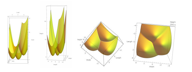
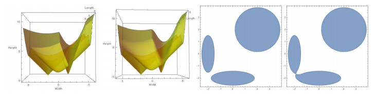
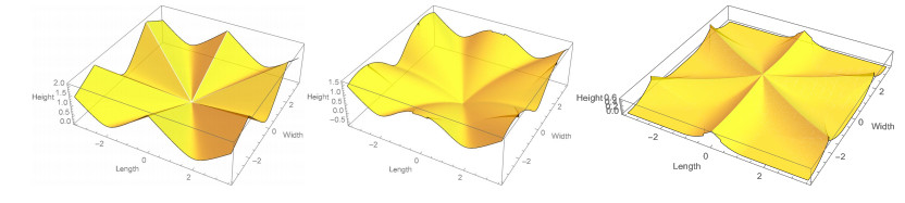
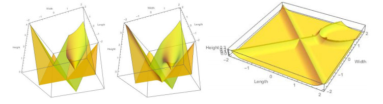
i) Let $ f:K\subseteq E\to E^\perp $ be an $ L $-Lipschitz mapping with $ 0\leq L\leq 1/\alpha $ and $ H_2(X) = \min\{ |P_EX-A_i|^2+\alpha|P_{E^\perp}X-f(A_i)|^2+\beta_i:\, i = 1, 2, \dots, k\} $, where $ \alpha > 0 $ is a control parameter, and
ii) $ H_1(X) = \alpha|P_{E^\perp}X|^2+\min\{\sqrt{|\mathcal{U}_i(P_EX-A_i)|^2+\gamma_i}: i = 1, 2, \dots, k\} $, where $ A_i\in E $ with $ U_i:E\to E $ invertible linear transforms for $ i = 1, 2, \dots, k $. If the control paramenter $ \alpha > 0 $ is sufficiently large, our quasiconvex lower bounds are 'tight' in the sense that near each 'well' the lower bound agrees with the original function, and our lower bound are of $ C^{1, 1} $. We also consider generalisations of our constructions to other simple geometrical multiwell models and discuss the implications of our constructions to the corresponding variational problems.
Citation: Ke Yin, Kewei Zhang. Some computable quasiconvex multiwell models in linear subspaces without rank-one matrices[J]. Electronic Research Archive, 2022, 30(5): 1632-1652. doi: 10.3934/era.2022082
In this paper we apply a smoothing technique for the maximum function, based on the compensated convex transforms, originally proposed by Zhang in [
i) Let $ f:K\subseteq E\to E^\perp $ be an $ L $-Lipschitz mapping with $ 0\leq L\leq 1/\alpha $ and $ H_2(X) = \min\{ |P_EX-A_i|^2+\alpha|P_{E^\perp}X-f(A_i)|^2+\beta_i:\, i = 1, 2, \dots, k\} $, where $ \alpha > 0 $ is a control parameter, and
ii) $ H_1(X) = \alpha|P_{E^\perp}X|^2+\min\{\sqrt{|\mathcal{U}_i(P_EX-A_i)|^2+\gamma_i}: i = 1, 2, \dots, k\} $, where $ A_i\in E $ with $ U_i:E\to E $ invertible linear transforms for $ i = 1, 2, \dots, k $. If the control paramenter $ \alpha > 0 $ is sufficiently large, our quasiconvex lower bounds are 'tight' in the sense that near each 'well' the lower bound agrees with the original function, and our lower bound are of $ C^{1, 1} $. We also consider generalisations of our constructions to other simple geometrical multiwell models and discuss the implications of our constructions to the corresponding variational problems.

| [1] |
K. Zhang, Compensated convexity and its applications, Ann. Inst. H. Poincaré Anal. Non Linéaire, 25 (2008), 743–771. https://doi.org/10.1016/j.anihpc.2007.08.001 doi: 10.1016/j.anihpc.2007.08.001

|
| [2] | Y. Chen, X. Ye, Projection onto a simplex, arXiv preprint, (2011), arXiv: 1101.6081. |
| [3] |
C. W. Combettes, S. Pokutta, Complexity of linear minimization and projection on some sets, Oper. Res. Lett., 49 (2021), 565–571. https://doi.org/10.1016/j.orl.2021.06.005 doi: 10.1016/j.orl.2021.06.005
|
| [4] |
L. Condat, Fast projection onto the simplex and the $l_1$ ball, Math. Program., 158 (2016), 575–585. https://doi.org/10.1007/s10107-015-0946-6 doi: 10.1007/s10107-015-0946-6
|
| [5] |
E. Y. Pee, J. O. Royset, On solving large-scale finite minimax problems using exponential smoothing, J. Optim. Theory Appl., 148 (2011), 390–421. https://doi.org/10.1023/B:JOTA.0000006685.60019.3e doi: 10.1023/B:JOTA.0000006685.60019.3e
|
| [6] | K. Zhang, Convex analysis based smooth approximations of maximum functions and squared distance functions, J. Nonlinear Convex Anal., 9 (2008), 379–406. |
| [7] |
K. Zhang, A. Orlando, E. Crooks, Compensated convexity and Hausdorff stable geometric singularity extractions, Math. Models Methods Appl. Sci., 25 (2015), 747–801. https://doi.org/10.1142/S0218202515500189 doi: 10.1142/S0218202515500189
|
| [8] |
K. Zhang, A. Orlando, E. Crooks, Compensated convexity and Hausdorff stable extraction of intersections for smooth manifolds, Math. Models Methods Appl. Sci., 25 (2015), 839–873. https://doi.org/10.1142/S0218202515500207 doi: 10.1142/S0218202515500207
|
| [9] |
K. Zhang, E. Crooks, A. Orlando, Compensated convexity, multiscale medial axis maps and sharp regularity of the squared distance function, SIAM J. Math. Anal., 47 (2015), 4289–4331. https//doi.org/10.1137/140993223 doi: 10.1137/140993223
|
| [10] |
K. Zhang, E. Crooks, A. Orlando, Compensated convexity methods for approximations and interpolations of sampled functions in Euclidean spaces: theoretical foundations, SIAM J. Math. Anal., 48 (2016), 4126–4154. https://doi.org/10.1137/15M1045673 doi: 10.1137/15M1045673
|
| [11] |
K. Zhang, E. Crooks, A. Orlando, Compensated convexity methods for approximations and interpolations of sample functions in Euclidean spaces: Applications to sparse data, contour lines and inpainting, SIAM J. Imaging Sci., 11 (2018), 2368–2428. https://doi.org/10.1137/17M116152X doi: 10.1137/17M116152X
|
| [12] | C. B. Morrey Jr, Multiple Integrals in the Calculus of Variations, Springer-Verlag, New York, 1966. https://doi.org/10.1007/978-3-540-69952-1 |
| [13] | B. Dacorogna, Direct Methods in the Calculus of Variations, 2$^{nd}$ edition, Springer-Verlag, New York, 1989. https://doi.org/10.1007/978-0-387-55249-1 |
| [14] |
J. M. Ball, Convexity conditions and existence theorems in nonlinear elasticity, Arch. Rational Mech. Anal., 63 (1977), 337–403. https://doi.org/10.1007/BF00279992 doi: 10.1007/BF00279992
|
| [15] |
E. Acerbi, N. Fusco, Semicontinuity problems in the calculus of variations, Arch. Rational Mech. Anal., 86 (1984), 125–145. https://doi.org/10.1007/BF00275731 doi: 10.1007/BF00275731
|
| [16] |
J. M. Ball, R. D. James, Fine phase mixtures as minimizers of energy, Arch. Rational Mech. Anal., 100 (1987), 13–52. https://doi.org/10.1007/BF00281246 doi: 10.1007/BF00281246
|
| [17] |
J. M. Ball, R. D. James, Proposed experimental tests of a theory of fine microstructures and the two-well problem, Philos. Trans. R. Soc. A, 338 (1992), 389–450. https://doi.org/10.1098/rsta.1992.0013 doi: 10.1098/rsta.1992.0013
|
| [18] |
V. Šverák, Quasiconvex functions with subquadratic growth, Proc. Royal Soc. London Ser. A, 433 (1991), 723–F725. https://doi.org/10.1098/rspa.1991.0073 doi: 10.1098/rspa.1991.0073
|
| [19] | K. Zhang, A construction of quasiconvex functions with linear growth at infinity, Ann. Scuola Norm. Sup. Pisa Cl. Sci., 19 (1992), 313–326. |
| [20] |
R. V. Kohn, The relaxation of a double-well energy, Cont. Mech. Therm., 3 (1991), 981–1000. https://doi.org/10.1007/BF01135336 doi: 10.1007/BF01135336
|
| [21] |
N. B. Firoozye, Optimal use of the translation method and relaxations of variational problems, Comm. Pure Appl. Math., 44 (1991), 643–678. https://doi.org/10.1002/cpa.3160440603 doi: 10.1002/cpa.3160440603
|
| [22] |
K. Bhattacharya, N. B. Firoozye, R. D. James, R.V. Kohn, Restrictions on microstructures, Proc. Royal Soc. Edinb. - A, 124 (1994), 843–878. https://doi.org/10.1017/S0308210500022381 doi: 10.1017/S0308210500022381
|
| [23] | M. Giaquinta, Introduction to regularity theory for nonlinear elliptic systems, Lectures in Mathematics ETH Zürich, Birkhüser Verlag, Basel, 1993. https://doi.org/10.1007/978-88-7642-443-4 |
| [24] |
A. A. Ahmadi, A. Olshevsky, P. Parrilo, J. N. Tsitsiklis, NP-hardness of deciding convexity of quartic polynomials and related problems, Math. Program., 137 (2013), 453–476. https://doi.org/10.1007/s10107-011-0499-2 doi: 10.1007/s10107-011-0499-2
|
| [25] |
G. Dolzmann, Numerical computation of rank-one convex envelopes, SIAM J. Numer. Anal., 36 (1999), 1621–1635. https://doi.org/10.1137/S0036142997325581 doi: 10.1137/S0036142997325581
|
| [26] |
K. Zhang, E. Crooks, A. Orlando, Compensated convexity on bounded domains, mixed Moreau envelopes and computational methods, Appl. Math. Model., 94 (2021), 688–720. https://doi.org/10.1016/j.apm.2021.01.040 doi: 10.1016/j.apm.2021.01.040
|
| [27] |
K. Zhang, Mountain pass solutions for a double-well energy, J. Differ. Equ., 182 (2002), 490–510. https://doi.org/10.1006/jdeq.2001.4113 doi: 10.1006/jdeq.2001.4113
|
| [28] | K. Zhang, An elementary derivation of the generalized Kohn-Strang relaxation formulae, J. Convex Anal., 9 (2002), 269–285. |
Figures(4)
Ke Yin, Kewei Zhang. Some computable quasiconvex multiwell models in linear subspaces without rank-one matrices[J]. Electronic Research Archive, 2022, 30(5): 1632-1652. doi: 10.3934/era.2022082


 DownLoad: