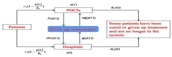
Figure 1.
Schematic diagram of China's medical two-way referral system.


In this article, we firstly establish a nonlinear population dynamical model to describe the changes and interaction of the density of patient population of China's primary medical institutions (PHCIs) and hospitals in China's medical system. Next we get some sufficient conditions of existence of positive singularity by utilising homotopy invariance theorem of topological degree. Meanwhile, we study the qualitative properties of positive singularity based on Perron's first theorem. Furthermore, we briefly analyze the significance and function of the mathematical results obtained in this paper in practical application. As verifications, some numerical examples are ultimately exploited the correctness of our main results. Combined with the numerical simulation results and practical application, we give some corresponding suggestions. Our research can provide a certain theoretical basis for government departments to formulate relevant policies.
Citation: Xiaoxia Zhao, Lihong Jiang, Kaihong Zhao. A nonlinear population dynamics model of patient diagnosis and treatment involving in two level medical institutions and its qualitative analysis of positive singularity[J]. Mathematical Biosciences and Engineering, 2022, 19(3): 2575-2591. doi: 10.3934/mbe.2022118
| [1] | Pengyan Liu, Hong-Xu Li . Global behavior of a multi-group SEIR epidemic model with age structure and spatial diffusion. Mathematical Biosciences and Engineering, 2020, 17(6): 7248-7273. doi: 10.3934/mbe.2020372 |
| [2] | Chang-Yuan Cheng, Shyan-Shiou Chen, Xingfu Zou . On an age structured population model with density-dependent dispersals between two patches. Mathematical Biosciences and Engineering, 2019, 16(5): 4976-4998. doi: 10.3934/mbe.2019251 |
| [3] | Yansong Pei, Bing Liu, Haokun Qi . Extinction and stationary distribution of stochastic predator-prey model with group defense behavior. Mathematical Biosciences and Engineering, 2022, 19(12): 13062-13078. doi: 10.3934/mbe.2022610 |
| [4] | Xin-You Meng, Yu-Qian Wu . Bifurcation analysis in a singular Beddington-DeAngelis predator-prey model with two delays and nonlinear predator harvesting. Mathematical Biosciences and Engineering, 2019, 16(4): 2668-2696. doi: 10.3934/mbe.2019133 |
| [5] | Eduardo Ibargüen-Mondragón, Lourdes Esteva, Edith Mariela Burbano-Rosero . Mathematical model for the growth of Mycobacterium tuberculosis in the granuloma. Mathematical Biosciences and Engineering, 2018, 15(2): 407-428. doi: 10.3934/mbe.2018018 |
| [6] | Nikolaos Kazantzis, Vasiliki Kazantzi . Characterization of the dynamic behavior of nonlinear biosystems in the presence of model uncertainty using singular invariance PDEs: Application to immobilized enzyme and cell bioreactors. Mathematical Biosciences and Engineering, 2010, 7(2): 401-419. doi: 10.3934/mbe.2010.7.401 |
| [7] | Tewfik Sari, Miled El Hajji, Jérôme Harmand . The mathematical analysis of a syntrophic relationship between two microbial species in a chemostat. Mathematical Biosciences and Engineering, 2012, 9(3): 627-645. doi: 10.3934/mbe.2012.9.627 |
| [8] | Weicheng Chen, Zhanping Wang . Stability of a class of nonlinear hierarchical size-structured population model. Mathematical Biosciences and Engineering, 2022, 19(10): 10143-10159. doi: 10.3934/mbe.2022475 |
| [9] | Miled El Hajji, Frédéric Mazenc, Jérôme Harmand . A mathematical study of a syntrophic relationship of a model of anaerobic digestion process. Mathematical Biosciences and Engineering, 2010, 7(3): 641-656. doi: 10.3934/mbe.2010.7.641 |
| [10] | Peter W. Bates, Jianing Chen, Mingji Zhang . Dynamics of ionic flows via Poisson-Nernst-Planck systems with local hard-sphere potentials: Competition between cations. Mathematical Biosciences and Engineering, 2020, 17(4): 3736-3766. doi: 10.3934/mbe.2020210 |
In this article, we firstly establish a nonlinear population dynamical model to describe the changes and interaction of the density of patient population of China's primary medical institutions (PHCIs) and hospitals in China's medical system. Next we get some sufficient conditions of existence of positive singularity by utilising homotopy invariance theorem of topological degree. Meanwhile, we study the qualitative properties of positive singularity based on Perron's first theorem. Furthermore, we briefly analyze the significance and function of the mathematical results obtained in this paper in practical application. As verifications, some numerical examples are ultimately exploited the correctness of our main results. Combined with the numerical simulation results and practical application, we give some corresponding suggestions. Our research can provide a certain theoretical basis for government departments to formulate relevant policies.
The country's basic medical system is closely related to people's life. Some scholars and media [1,2,3] have conducted extensive and in-depth discussions and researches on this problem. Through unremitting efforts, the Chinese government has established primary medical institutions (PHCIs) and hospitals to meet the medical needs of urban and rural people. For relevant research and discussion, the readers refer to references [4,5,6]. PHCIs mainly treat and recover patients with common and frequently occurring diseases such as cold, headache and fever, while hospitals mainly receive patients with serious diseases that cannot be treated by PHCIs [7,8].
Although China has a large number of PHCIs and hospitals, many patients living in remote areas face medical difficulties and expensive medical expenses [9]. This situation is mainly caused by the unbalanced allocation of medical resources in China. The hospitals have more high-quality medical resources than PHCIs [10]. In addition, Chinese residents are free to choose medical institutions for medical treatment. Many patients choose to go to hospitals with better medical conditions rather than PHCIs. This has resulted in hospital medical congestion and shortage of medical resources, while PHCIs is semi-idle. For patients, it also increases the difficulty and cost of medical treatment [11,12,13,14]. The 2019 China Health Statistics Yearbook [15,16] shows that the average number of patients in hospitals and PHCI is 202.3 and 0.307 respectively.
In the medical system reform proposed by the Chinese government in 2019, it is pointed out that the two-way referral system can realize the sharing of medical resources among medical institutions and solve the problem of unbalanced distribution of medical resources among regions to a certain extent [17,18]. The so-called two-way referral is that the PHCIs transfer the patients who are difficult to diagnose and treat to the hospital, and the hospital transfers the patients who are getting better to PHCIs. In addition, using telemedicine, hospitals can help PHCIs improve their diagnosis and treatment ability, and promote more patients to choose PHCIs for treatment. For example, hospitals improve the treatment level of PHCIs by means of diagnostic suggestions and distance education, so as to promote patients to choose PHCIs for treatment. This saves a lot of medical time and cost for patients [19,20,21]. Thereby, exploring the application of two-way referral in the medical system is very important for patients' reasonable medical treatment and the healthy development of China's medical system.
Since medical resources are limited, if we assume that patients choose medical institutions strictly by the division of labor of medical institutions, then PHCIs and hospital diagnosis and treatment density conform to the logistic block growth law, which means that they will not grow indefinitely when the number of visits to medical institutions reaches a certain level. Next, we'll establish a nonlinear population dynamics model to reveal the relationship of patient visit rates of China's PHCIs and hospitals in the two-way referral system in this paper, as shown in Figure 1.
We use the non-negative, continuous and differentiable function x(t) and y(t) to represent the visiting population density in PHCIs and hospitals at time t. Denote r1>0 and r2>0 be their inherent increase rate, which is positively related to the population growth rate. k1>0 and k2>0 represent the maximum visiting capacity of PHCIs and hospitals, which is positively correlated with the comprehensive capabilities of the respective medical institutions. So, the change of the visiting population density per unit time in China's medical system can be expressed as:
| {˙x(t)=r1x(t)(1−x(t)k1),˙y(t)=r2y(t)(1−y(t)k2). | (1.1) |
The model (1.1) is a typical logistic population dynamics model. This model reflects the change law of the visiting population density in PHCIs and hospitals without the influence of external factors. Meanwhile, the visiting population in PHCIs and hospitals is independent of each other and does not flow. Obviously, this model is unreasonable. Therefore, we need to modify the model (1.1). In the two-way-referral system, we use a function f(x(t))>0 to represent the density of patients who cannot be treated by PHCIs, and mf(x(t)) stands for the population density of patients who lost to PHCIs and eventually went to hospitals for treatment. Since the diagnosis and treatment ability of PHCIs and hospitals has been improved by the implementation of telemedicine. And in order to relieve the pressure of hospital treatment, the government transfers some hospital patients to PHCIs. We assume that the function g(y(t)) is the adjusting patient population density to PHCIs and ng(y(t)) stands for the population density of patients who leave to hospitals and eventually went to PHCIs for treatment. The constants m and n (0<m,n≤1) are regarded as the conversion rate. We use d1>0 and d2>0 to represent the churn rate of the density of diagnosis and treatment in PHCIs and hospitals, which reduces the number of visits to medical institutions. They are positively correlated with population mortality and the number of people who have given up treatment. Thus, the model (1.1) can be modified as follows:
| {˙x(t)=r1x(t)(1−x(t)k1)−d1x(t)−f(x(t))+ng(y(t)),˙y(t)=r2y(t)(1−y(t)k2)−d2y(t)+mf(x(t))−g(y(t)). | (1.2) |
Remark 1.1. The model (1.2) reflects the mutual flow of visiting population between PHCIs and hospitals by the terms f(x(t)) and mf(x(t)). The terms g(y(t)) and ng(y(t)) also reflect the regulatory role of government departments. The terms d1x(t) and d2y(t) reflect the curative effects of PHCIs and hospitals. So the model (1.2) is a relatively reasonable mathematical model. Unfortunately, due to the lack of data on the flow of visiting population and the government's regulation of visiting population, we can't give the expressions and relevant information of the function f(x(t)) and g(y(t)). This limits the application of the model (1.2).
In this paper, we mainly study the existence of positive singularity and its qualitative analysis for the model (1.2). The remainder of the paper is structured as follows. In Section 2, we obtain the existence of positive singularity and its qualitative analysis. In Section 3, some examples and its simulations are illustrated the effectiveness of our results. We briefly summarize the used methods and obtained results in Section 4.
In this section, we will show that model (1.2) exists at least positive singularity and analyze its qualitative behaviors. Let X=C1(R,R+)×C1(R,R+), for all (x,y)T∈X, define the norm ‖(x,y)T‖=max{supt∈R|x(t)|,supt∈R|x(t)|}. It is easy to verify X is a Banach space with this norm.
Theorem 2.1. If the following conditions (A1)-(A2) hold, then model (1.2) at least exists one positive singularity E=(x0,y0)T.
(A1) Assume that the functions f,g∈C(R,R+), and there exist some constants L1,L2>0 such that
| |f(u)−f(v)|≤L1|u−v|,|g(u)−g(v)|≤L2|u−v|,∀u,v∈R,u≠v. |
(A2) r1−d1−L1−nL2>0 and r2−d2−mL1−L2>0.
Let
| h(x,y)=(h1(x,y),h2(x,y))T=(0,0)T=θ, | (2.1) |
where
| {h1(x,y)=r1x(1−xk1)−d1x−f(x)+ng(y),h2(x,y)=r2y(1−yk2)−d2y+mf(x)−g(y). |
Obviously, the solutions of model (2.1) are the singularities of model (1.2).
Take Ω={(x,y)T∈X:‖(x,y)T‖≤R0}, where R0 satisfies
| |f(0)|+n|g(0)|+r1k1r1−d1−L1−nL2<R0,m|f(0)|+|g(0)|+r2k2r2−d2−mL1−L2<R0. | (2.2) |
Define homotopic mapping
| H(x,y,λ)=(H1(x,y,λ),H2(x,y,λ))T=λh(x,y)+(1−λ)(x,y)T,λ∈[0,1]. | (2.3) |
For all (x,y)∈∂Ω, according to (A1), (A2) and model (2.2), and noticing that x(t)≤k1 and y(t)≤k2, we have
| |H1(x,y,λ)|=|λ[r1x(1−xk1)−d1x−f(x)+ng(y)]+(1−λ)x|=|λ[r1x(1−xk1)−d1x−[f(x)−f(0)]+f(0)+n[g(y)−g(0)]+ng(0)]+(1−λ)x|≥λ(r1−d1−L1−nL2)R0−|f(0)|−n|g(0)|−r1k1+(1−λ)R0>0,λ∈[0,1]. | (2.4) |
and
| |H2(x,y,λ)|=|λ[r2y(1−yk2)−d2y−g(y)+mf(x)]+(1−λ)y|=|λ[r2y(1−yk2)−d2y−[g(y)−g(0)]+g(0)+m[f(x)−f(0)]+mf(0)]+(1−λ)y|≥λ(r2−d2−L2−mL2)R0−|g(0)|−m|f(0)|−r2k2+(1−λ)R0>0,λ∈[0,1]. | (2.5) |
Models (2.4) and (2.5) indicate that
| H(x,y,λ)≠(0,0)T,∀(x,y)T∈∂Ω,λ∈[0,1]. |
Therefore, we derive from homotopy invariance theorem [22] that
| d(h,Ω,θ)=d(H(x,y,1),Ω,θ)=d(H(x,y,0),Ω,θ)=1, |
where d(h,Ω,θ) denotes topological degree [23]. By topological degree theory, we know that model (2.1) has at least one solution (x0,y0)T∈Ω. Namely, model (1.2) has at least positive singularity E=(x0,y0)T.
Next we shall discuss the qualitative properties of positive singularity (x0,y0)T of model (1.2). Consider the following nonlinear system and its corresponding linear system
| {˙x(t)=ax+by+ϕ(x,y),˙y(t)=cx+dy+ψ(x,y), | (2.6) |
and
| {˙x(t)=ax+by,˙y(t)=cx+dy, | (2.7) |
where a,b,c and d are all real number, ϕ(0,0)=ψ(0,0)=0. Obviously, O(0,0) is a singularity of models (2.6) and (2.7). The following lemma is important.
Lemma 2.1. (Perron's first theorem [24]) Assume that ϕ(x,y) and ψ(x,y) satisfy two conditions as follows:
(i) ϕ(x,y) and ψ(x,y) exist continuous first-order partial derivativesin the domain of singularity O(0,0);
(ii) ϕ(x,y)=o(r), ψ(x,y)=o(r), r=√x2+y2.
If O(0,0) is the focus, normal node or saddle point of linear model (2.7), then O(0,0) is also a singularity of the same type for nonlinear model (2.6).
In order to discuss the qualitative properties of positive singularity E=(x0,y0) of model (1.2), we need to make the following assumptions.
(A3) Assume that the functions f,g:R→R+ are derivative, namely, for all u∈R, f′(u) and g′(u) exist.
If (A3) holds, then corresponding linear system of model (1.2) is read by
| (˙x˙y)=(a11a12a21a22)(x−x0y−y0), | (2.8) |
where a11=r1−d1−2r1k1x0−f′(x0), a12=ng′(y0), a21=mf′(x0), a22=r2−d2−2r2k2y0−g′(y0). And the characteristic equation of the model (2.8) is written as
| |λ−a11−a12−a21λ−a22|=λ2−(a11+a22)λ+(a11a22−a12a21)=0. | (2.9) |
By (A3), in the neighborhood of E=(x0,y0), we have
| f(x)−f(x0)=f′(x0)(x−x0)+o((x−x0)), | (2.10) |
| g(y)−g(y0)=g′(y0)(y−y0)+o((y−y0)), | (2.11) |
where limx→x0o((x−x0))x−x0=0, limy→y0o((y−y0))y−y0=0. And the conditions (A1) and (A2) are changed as
(A1)′ |f(x)−f(x0)|≤|f′(x0)||x−x0|,|g(y)−f(y0)|≤|g′(y0)||y−y0|.
(A2)′ r1−d1−|f′(x0)|−n|g′(y0)|>0 and r2−d2−m|f′(x0)|−|g′(y0)|>0.
Theorem 2.2. Assume that (A3) holds, then the following assertions hold:
(1) If a11+a22<0 and Δ=(a11−a22)2+4a12a21<0 hold, then E=(x0,y0) is a stable focus of system (1.2).
(2) If a11+a22>0 and Δ=(a11−a22)2+4a12a21<0 hold, then E=(x0,y0) is an unstable focus of system (1.2).
When a11+a22≠0 and Δ=(a11−a22)2+4a12a21<0 hold, the characteristic model (2.9) has a pair of conjugate complex roots λ1 and λ2
| λ1=a11+a22+i√−Δ2,λ2=a11+a22−i√−Δ2. |
When a11+a22<0 holds, λ1 and λ2 have negative real part. So E=(x0,y0) is a stable focus of Eq (2.1). When a11+a22>0 holds, λ1 and λ2 have positive real part. So E=(x0,y0) is an unstable focus of model (2.1).
From models (2.10) and (2.11), we have
| ϕ(x−x0,y−y0)=−r1k1(x−x0)2+o((x−x0)), | (2.12) |
and
| ψ(x−x0,y−y0)=−r2k2(y−y0)2+o((y−y0)). | (2.13) |
Let x−x0=rcosθ, y−y0=rsinθ, then we obtain r=√(x−x0)2+(y−y0)2 and
| limr→0+ϕ(x−x0,y−y0)=limr→0+[−r1k1(x−x0)2+o((x−x0))]=limr→0+[−r1k1r2cos2θ+o(r)]=0, | (2.14) |
and
| limr→0+ψ(x−x0,y−y0)=limr→0+[−r2k2(y−y0)2+o((y−y0))]=limr→0+[−r2k2r2sin2θ+o(r)]=0. | (2.15) |
Thus both (i) and (ii) are true. By Lemma 1, we know that E=(x0,y0) is also a stable focus when a11+a22<0 and Δ=(a11−a22)2+4a12a21<0 hold, or is an unstable focus for system (1.2) when a11+a22>0 and Δ=(a11−a22)2+4a12a21<0 hold.
Theorem 2.3. Assume that (A3) holds, then the following assertions hold:
(1) If a11+a22<0, a11a22−a12a21>0 and Δ=(a11−a22)2+4a12a21>0 hold, then E=(x0,y0) is a stable normal node of system (1.2).
(2) If a11+a22>0, a11a22−a12a21>0 and Δ=(a11−a22)2+4a12a21>0 hold, then E=(x0,y0) is an unstable normal node of system (1.2).
When Δ=(a11−a22)2+4a12a21>0, the characteristic Eq (2.9) have two different real roots λ1 and λ2
| λ1=a11+a22+√Δ2,λ2=a11+a22−√Δ2. |
When a11+a22<0 and a11a22−a12a21>0, then λ1<0 and λ2<0. So E=(x0,y0) is a stable normal node of model (2.1). When a11+a22>0 and a11a22−a12a21>0, then λ1>0 and λ2>0. So E=(x0,y0) is an unstable normal node of model (2.1). In view of Lemma 1, models (2.14) and (2.15), we conclude that E=(x0,y0) is also a stable normal node when a11+a22<0, a11a22−a12a21>0 and Δ=(a11−a22)2+4a12a21>0 hold, or is an unstable normal node for system (1.2) when a11+a22>0, a11a22−a12a21>0 and Δ=(a11−a22)2+4a12a21>0 hold.
Theorem 2.4. Assume that (A3) holds. If a11a22−a12a21<0 and Δ=(a11−a22)2+4a12a21>0 hold, then E=(x0,y0) is a saddle point of model (1.2).
When Δ=(a11−a22)2+4a12a21>0, the characteristic model (2.9) have two different real roots λ1 and λ2
| λ1=a11+a22+√Δ2,λ2=a11+a22−√Δ2. |
When a11a22−a12a21<0, then λ1λ2<0. So E=(x0,y0) is a saddle point of model (2.1). It follows from Lemma 1, models (2.14) and (2.15) that E=(x0,y0) is also a saddle point of model (1.2).
Next, we discuss the simplest special case of model (1.2). Let f(x)=c1x, g(y)=c2y, c1,c2>0, then model (1.2) is changed into
| {˙x(t)=r1x(t)(1−x(t)k1)−d1x(t)−c1x(t)+nc2y(t),˙y(t)=r2y(t)(1−y(t)k2)−d2y(t)+mc1x(t)−c2y(t). | (2.16) |
The positive singularity E(x0,y0) of model (2.16) is determined by the following algebraic equation
| {(r1−d1−c1)x−r1k1x2+nc2y=0,(r2−d2−c2)y−r2k2y+mc1x=0. | (2.17) |
Then we have a11=r1−d1−c1−2r1k1x0, a12=nc2, a21=mc1, a22=r2−d2−c2−2r2k2y0, Δ>0, a11+a22=−mnc1c2<0. Thus, only (1) of Theorems 2.3 and 2.4 hold. In fact, we have the following results.
Corollary 2.1. If (r1−d1−c1)+(r2−d2−c2)<2(r1k1+r2k2) and (r1−d1−c1)r1k1+(r2−d2−c2)r2k2≥34(r1−d1−c1)(r2−d2−c2) hold, then E=(x0,y0) is a stable normal node of system (2.16).
Corollary 2.2. If (r1−d1−c1)r1k1+(r2−d2−c2)r2k2<34(r1−d1−c1)(r2−d2−c2) holds, then E=(x0,y0) is a saddle point of system (2.16).
(1) Analysis and discussion of practical significance of positive singularity and its stability. In practice, the positive singularity E of model (1.2) represents the population density of patients when the number of patients in a PHCI and hospital tends to be stable after a long period of time. The value of singularity can help PHCI and hospital managers make more correct decisions in terms of the number of medical staff employed, the number of wards and beds, the grade and number of medical devices purchased, and the number of drugs purchased and stored, so as to avoid unnecessary waste. In a word, this value can be used as a reference for measuring the size of PHCIs and hospitals. The national health administration can also manage and allocate funds to PHCIs and hospitals based on the value of singularity. Therefore, the stability of positive singularity is very important. In mathematical theory, the stable singularity will not change greatly due to external interference, such as the change of initial value and parameter fluctuation in the equation. The case of unstable singularity is just the opposite. Therefore, in practical application, people prefer that the singularity of the model is stable, which is of great benefit to them to make correct decisions.
(2) Analysis and discussion of specific parameters and their relationship in model (1.2). r1 and r2 measure a natural increase in the number of patients in each PHCI and hospital without competition from other medical institutions, respectively. The values of r1 and r2 mainly depend on the population in their jurisdiction. k1 and k2 measure the maximum number of patients each PHCI and hospital, which mainly depends on the size of clinics and hospitals. d1 and d2 measure the number of patients cured in PHCIs and hospitals, which mainly depends on their size and medical level. 0≤m,n≤1 indicate the proportion of patients who left the PHCI (or hospital) and chose the hospital (or PHCI). The exact values of these parameters are generally difficult to determine. Generally, their approximate values can be obtained by least square fitting of relevant data for many years. It is more meaningful to consider the stable singularity in practical application. Therefore, the assertion (1) and inequality relations satisfied by parameters of Theorems 2.2 to 2.3 and Corollaries 2.1 to 2.2 are of practical significance. In the model (2.16), the parameters m and n have no effect on the singularity.
This section illustrates the rationality and effectiveness of our mathematical theoretical results through some examples and numerical simulation. Combined with the simulation results, some practical applications are analyzed and discussed.
Example 1. Consider the following nonlinear generalized patient diagnosis and treatment population dynamics model involving in two level medical institutions
| {˙x(t)=r1x(t)(1−x(t)k1)−d1x(t)−f(x(t))+ng(y(t)),˙y(t)=r2y(t)(1−y(t)k2)−d2y(t)+mf(x(t))−g(y(t)), | (3.1) |
Case 1. Let r1=5, r2=3, k1=8, k2=10, d1=0.4, d2=0.3, m=0.8, n=0.7, f(x)=ex, g(y)=ey. By calculations, we know that the positive singularity of (3.1) is E=(x0,y0), x0≈0.0047, y0≈0.0829. And a11≈3.5894, a22≈1.5638, a12≈0.8038, a21≈0.7605, a11+a22≈5.1532>0, a11a22−a12a21≈5.0018>0, Δ=(a11−a22)2+4a12a21≈6.1989>0, λ1≈3.8561>0, λ2≈1.2971>0. So we conclude from Theorem 2.3 that the positive singularity E=(0.0668,0.0884) is an unstable normal node. The phase portrait near the singularity E=(0.0668,0.0884) is shown as Figure 2. The evolutions of patient density x(t) and y(t) over time with different initial values are shown as Figures 3 and 4.


Analysis and discussion: In Case 1, it is easily seen from Figure 2 that E=(0.0668,0.0884) is a unstable normal node, which verifies that our theoretical outcomes are correct. Moreover, from Figures 3 and 4, we see that model (3.1) has another positive singularity E∗, which value is E∗=(3.3353,3.3372) by numerical calculation, and E∗ is asymptotic stable. In fact, our existence theorem of positive singularity only guarantees the existence of at least one positive singularity, but it does not guarantee uniqueness. For practical application, the number of patients lost from PHCI decreases sharply with exponential function ex(t), and the government medical management institutions also regulate with exponential function ey(t), which can achieve a certain balance. Because the cure rates of PHCI and hospitals are low, only d1=0.4 and d2=0.3 respectively, the population density of patients in PHCI and hospitals is only kept in a very low state E=(0.0668,0.0884), and this state is extremely unstable. Meanwhile, the PHCI and hospital as a whole have also lost some patients to medical institutions in other communities, which is reflected in 1−m=0.2 and 1−n=0.3. We suggest that the PHCI and hospital improve the level of diagnosis and treatment to increase the cure rate and ensure that patients in the community do not lose. Finally, the population density of patients in PHCI and hospital will reach a stable balance E∗=(3.3353,3.3372).
Case 2. Let r1=0.4, r2=0.3, k1=5, k2=8, d1=0.3, d2=0.2, m=0.9, n=0.6, f(x)=0.4x, g(y)=0.5y. By calculations, we know that the positive singularity of (3.1) is E=(x0,y0), x0≈0.3366, y0≈0.3117. And a11≈−0.3539, a22≈−0.4234, a12=0.36, a21≈0.3, a11+a22≈−0.7773<0, a11a22−a12a21≈0.0418>0, Δ=(a11−a22)2+4a12a21≈0.4368>0, λ1≈−0.0582<0, λ2≈−0.7191<0. So we conclude from Theorem 2.3 that the positive singularity E=(0.0334,0.0412) is a stable normal node. The phase portrait near the singularity E=(0.0334,0.0412) is shown as Figure 5. The evolutions of patient density x(t) and y(t) over time with different initial values are shown as Figures 6 and 7.


Analysis and discussion: In Case 2, it is easily seen from Figures 5 and 4 that E=(0.0334,0.0412) is a stable normal node, which verify that our theoretical outcomes are correct. For practical application, the number of patients lost from PHCI decreases with linear function 0.4x(t), and the government medical management institutions also regulate with linear function 0.5y(t), which can achieve a certain balance. Because the cure rates of PHCI and hospitals are low, only d1=0.3 and d2=0.2 respectively, the population density of patients in PHCI and hospitals is only kept in a very low state E=(0.0334,0.0412). Meanwhile, the PHCI and hospital as a whole have also lost some patients to medical institutions in other communities, which is reflected in 1−m=0.1 and 1−n=0.4. Our suggestions and warnings are that the PHCI and hospital improve the level of diagnosis and treatment to increase the cure rate and ensure that patients in the community do not lose. At the same time, the medical management department should strengthen control and adjustment. Otherwise, the PHCI and hospital will be closed without patients.
Case 3. Let r1=1, r2=1, k1=8, k2=10, d1=0.4, d2=0.3, m=0.8, n=0.7, f(x)=ex, g(y)=ey. By calculations, we know that the positive singularity of (3.1) is E=(x0,y0), x0≈0.4188, y0≈0.0788. And a11≈−1.0248, a22≈−0.3977, a12=0.8038, a21≈0.7605, a11a22−a12a21≈−0.2037<0, Δ=(a11−a22)2+4a12a21≈2.8384>0, λ1≈0.1311>0, λ2≈−1.5536<0. So we conclude from Theorem 2.4 that the positive singularity E=(0.0418,0.0788) is a saddle point. The phase portrait near the singularity E=(0.0418,0.0788) is shown as Figure 8. The evolutions of patient density x(t) and y(t) over time with different initial values are shown as Figures 9 and 10.


Analysis and discussion: In Case 3, it is easily seen from Figures 8–10 that E=(0.4188,0.0788) is a saddle point, which verify that our theoretical outcomes are correct. For practical application, the number of patients lost from PHCI decreases sharply with exponential function ex(t), and the government medical management institutions also regulate with exponential function ey(t), but which does not achieve a certain balance. Because the cure rates of PHCI and hospital are low, only d1=0.4 and d2=0.3 respectively. Meanwhile, the PHCI and hospital as a whole have also lost some patients to medical institutions in other communities, which is reflected in 1−m=0.2 and 1−n=0.3. The solutions starting from an initial value change independently. In this case, the number of patients in PHCI and hospital is very uncertain. This puzzles the development of PHCI and hospital and the investment of medical expenses. We suggest that the PHCI, hospital and medical management department should deeply investigate and study the main causes of this situation, and make adjustments and governance, so that the system can be in a stable and balanced state.
Example 2: Consider the following simplest special case of model (1.2)
| {˙x(t)=r1x(t)(1−x(t)k1)−d1x(t)−c1x(t)+nc2y(t),˙y(t)=r2y(t)(1−y(t)k2)−d2y(t)+mc1x(t)−c2y(t). | (3.2) |
Let r1=1, k1=2, d1=0.4, c1=0.6, r2=1, k2=4, d2=0.6, c2=0.5, m=1, n=1. By a simple calculation, we get r1−c1−d1+r2−d2−c2=−0.1000, 2(r1k1+r2k2)=1.5000, (r1−d2−c1)r1k1+(r2−d2−c2)r2k2=0.7500, 34(r1−d1−c1)(r2−d2−c2)=0.7500. The positive singularity E=(1.2395,1.5363). Thus (1) of Corollary 2.1 hold, then the positive singularity E=(1.2395,1.5363) is a stable normal node. The phase portrait near the singularity E=(1.2395,1.5363) is shown as Figure 11. The evolutions of patient density x(t) and y(t) over time with different initial values are shown as Figures 12 and 13.


Analysis and discussion: It is easily seen from Figures 11–13 that E=(1.2395,1.5363) is a stable normal node, which verify that our theoretical outcomes are correct. For practical application, the number of patients lost from PHCI decreases with linear function 0.6x(t), and the government medical management institutions also regulate with linear function 0.5y(t), which can achieve a certain balance. Because the cure rates of PHCI and hospitals are higher arrival to d1=0.4 and d2=0.6 respectively. Meanwhile, the patients of PHCI and hospital don't lost, which is reflected in m=n=1. This makes the population density of patients in PHCI and hospital reach an ideal stable state E=(1.2395,1.5363). Our suggestion is that the PHCI and hospital improve the level of diagnosis and treatment to increase the cure rate.
Primary medical institutions and hospitals are the most important components of China's public medical system. However, due to the different conditions of medical resources, the number of patients they can treat is also different from each other. Studying the changes in the number of patients and their relationship can help government departments carry out macro-control. Therefore, we try to use calculus theory and method to establish dynamic equation model to study this problem. In this article, a nonlinear population dynamics model (1.2) is establish to describe the correlations of the density of patient population of China's primary medical institutions and hospitals. Some sufficient conditions are obtained for the existence of positive singularities and the existence of positive singularities as the focus, normal node and saddle point for this model. Some numerical simulations to verify the validity of our results. Combined with the numerical simulation results and practical application, we give some corresponding suggestions. Our research can provide a certain theoretical basis for government departments to formulate relevant policies. In addition, the condition that the positive singularities of the model are true centers or small focus is worth discussing in the future.
This work was supported by the National Natural Sciences Foundation of Peoples Republic of China under Grant (Nos. 71764035, 71864021). The authors would like to thank the anonymous referees for their useful and valuable suggestions.
All authors declare that they have no competing interests.
| [1] | The 19th National Congress of the Communist Party of China, Development of China's Public Health as an Essential Element of Human Rights, Available from: https://english.dbw.cn/system/2017/09/30/001228107.shtml. |
| [2] |
W. Yip, H. Fu, A. T. Chen, T. Zhai, W. Jian, R. Xu, et al., 10 years of health-care reform in China: progress and gaps in universal health coverage, Lancet, 394 (2019), 1192–1204. https://doi.org/10.1016/S0140-6736(19)32136-1. doi: 10.1016/S0140-6736(19)32136-1

|
| [3] |
L. Zhang, G. Cheng, S. Song, B. Yuan, W. Zhu, L. He, et al., Efficiency performance of China's health care delivery system, Int. J. Health Plan. Manage., 32 (2017), 254–263. https://doi.org/10.1002/hpm.2425. doi: 10.1002/hpm.2425
|
| [4] |
Q. Meng, A. Mills, L. Wang, Q. Han, What can we learn from China's health system reform? BMJ, 365 (2019), l2349. https://doi.org/10.1136/bmj.l2349. doi: 10.1136/bmj.l2349
|
| [5] |
Y. Niu, L. Zhang, T. Ye, Y. Yan, Y. Zhang, Can unsuccessful treatment in primary medical institutions influence patients' choice? A retrospective cluster sample study from China, BMJ Open, 9 (2019), e022304. https://doi.org/10.1136/bmjopen-2018-022304. doi: 10.1136/bmjopen-2018-022304
|
| [6] |
L. Li, H. Fu, China's health care system reform: Progress and prospects, Int. J. Health Plan. Manage., 32 (2017), 240–253. https://doi.org/10.1002/hpm.2424. doi: 10.1002/hpm.2424
|
| [7] |
X. Li, J. Lu, S. Hu, K. K. Cheng, J. De Maeseneeret, Q. Meng, et al., The primary health-care system in China, Lancet, 390 (2017), 2584–2594. https://doi.org/10.1016/S0140-6736(17)33109-4. doi: 10.1016/S0140-6736(17)33109-4
|
| [8] |
G. Ridic, S. Gleason, O. Ridic, Comparisons of health care systems in the United States, Germany and Canada, Mater. Sociomed., 24 (2012), 112–120. https://doi.org/10.5455/msm.2012.24.112-120. doi: 10.5455/msm.2012.24.112-120
|
| [9] |
J. Liu, H. Yin, T. Zheng, B. Ilia, X. Wang, R. Chen, et al., Primary health institutions preference by hypertensive patients: Effect of distance, trust and quality of management in the rural Heilongjiang province of China, BMC Health Serv. Res., 19 (2019), 852. https://doi.org/10.1186/s12913-019-4465-7. doi: 10.1186/s12913-019-4465-7
|
| [10] | U.S.-China Economic and Security Review Commission, China's healthcare system: addressing capacity shortfalls before and after COVID-19. https://www.uscc.gov/research/chinas-healthcare-system-addressing-capacityshortfalls-and-after-covid-19. |
| [11] |
T. Zhang, Y. Xu, J. Ren, L. Sun, C. Liu, Inequality in the distribution of health resources and health services in China: hospitals versus primary care institutions, Int. J. Equity Health, 42 (2017), doi.org/10.1186/s12939-017-0543-9. doi: 10.1186/s12939-017-0543-9
|
| [12] |
D. Blumenthal, W. Hsiao, Privatization and its discontents-the evolving Chinese health care system, N. Engl. J. Med., 353 (2005), 1165–1170. https://doi.org/10.1056/NEJMhpr051133. doi: 10.1056/NEJMhpr051133
|
| [13] |
S. Hu, S. Tang, Y. Liu, Y. Zhao, M. Escobar, D. De Ferranti, Reform of how health care is paid for in China: challenges and opportunities, Lancet, 372 (2008), 1846–1853. https://doi.org/10.1016/S0140-6736(08)61368-9. doi: 10.1016/S0140-6736(08)61368-9
|
| [14] |
S. Anand, V. Fan, J. Zhang, L. Zhang, Y. Ke, Z. Dong, et al., China's human resources for health: quantity, quality and distribution, Lancet, 372 (2008), 1774–1781. https://doi.org/10.1016/S0140-6736(08)61363-X. doi: 10.1016/S0140-6736(08)61363-X
|
| [15] | National Health Commission: China's Health Statistics Yearbook 2020, Peking Union Medical College Press, Beijing, 2020. Available from: https://www.yearbookchina.com/navibooklist-n3020013080-1.html?from=singlemessage. |
| [16] | China Society of Social Security, China's statistical communique on health development 2019, 2020. Available from: http://www.caoss.org.cn/sbnr.asp?id=1919. |
| [17] |
D. Wu, H. Gu, S. Gu, H. You, Individual motivation and social influence: a study of telemedicine adoption in China based on social cognitive theory, Health Policy Technol., 10 (2021), 100525. https://doi.org/10.1016/j.hlpt.2021.100525. doi: 10.1016/j.hlpt.2021.100525
|
| [18] |
J. Liu, S. Liu, T. Zheng, Y. Bi, Physicians' perspective of telemedicine during the COVID-19 in China: Qualitative survey study, JMIR Med. Inform., 9 (2021), e26463. https://doi.org/10.2196/26463. doi: 10.2196/26463
|
| [19] |
Y. Wang, B. Li, L. Liu, Telemedicine experience in China: Our response to the pandemic and current challenges, Front. Public Health, 8 (2020), 549669. https://doi.org/10.3389/fpubh.2020.549669. doi: 10.3389/fpubh.2020.549669
|
| [20] |
F. Cui, Q. Ma, X. He, Y. Zhai, J. Zhao, B. Chen, et al., Implementation and application of telemedicine in China: Cross-sectional study, JMIR Mhealth Uhealth, 8 (2020), e18426. https://doi.org/10.2196/18426. doi: 10.2196/18426
|
| [21] |
Y. Han, A. Li, A. Stevens, J. Xiao, J. Yu, Z. Jiang, Improving access to healthcare services through an indepth understanding of telemedicine in China, Value Health, 2 (2018), S20. https://doi.org/10.1016/j.jval.2018.07.157. doi: 10.1016/j.jval.2018.07.157
|
| [22] | S. Hu, Nonlinear Analysis Theory and Methods, Huazhong University of Science and Technology Press, Wuhan, 1996. |
| [23] | D. Guo, J. Sun, Z. Liu, Functional Methods of Nonlinear Ordinary Differential Equations, Shandong Science and Technology Press, Jinan, 1995. |
| [24] | J. Hale, Ordinary Differential Equations, John Wiley and Sons, New York, 1969. https://doi.org/10.2307/2316346. |
Figures(13)

Xiaoxia Zhao, Lihong Jiang, Kaihong Zhao. A nonlinear population dynamics model of patient diagnosis and treatment involving in two level medical institutions and its qualitative analysis of positive singularity[J]. Mathematical Biosciences and Engineering, 2022, 19(3): 2575-2591. doi: 10.3934/mbe.2022118

 DownLoad:
