A mathematical model of tumor-immune system interactions with an oncolytic virus therapy for which the immune system plays a twofold role against cancer cells is derived. The immune cells can kill cancer cells but can also eliminate viruses from the therapy. In addition, immune cells can either be stimulated to proliferate or be impaired to reduce their growth by tumor cells. It is shown that if the tumor killing rate by immune cells is above a critical value, the tumor can be eradicated for all sizes, where the critical killing rate depends on whether the immune system is immunosuppressive or proliferative. For a reduced tumor killing rate with an immunosuppressive immune system, that bistability exists in a large parameter space follows from our numerical bifurcation study. Depending on the tumor size, the tumor can either be eradicated or be reduced to a size less than its carrying capacity. However, reducing the viral killing rate by immune cells always increases the effectiveness of the viral therapy. This reduction may be achieved by manipulating certain genes of viruses via genetic engineering or by chemical modification of viral coat proteins to avoid detection by the immune cells.
Citation: G. V. R. K. Vithanage, Hsiu-Chuan Wei, Sophia R-J Jang. Bistability in a model of tumor-immune system interactions with an oncolytic viral therapy[J]. Mathematical Biosciences and Engineering, 2022, 19(2): 1559-1587. doi: 10.3934/mbe.2022072
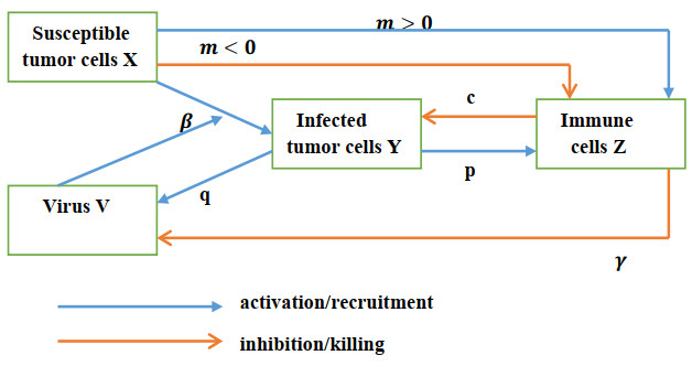
A mathematical model of tumor-immune system interactions with an oncolytic virus therapy for which the immune system plays a twofold role against cancer cells is derived. The immune cells can kill cancer cells but can also eliminate viruses from the therapy. In addition, immune cells can either be stimulated to proliferate or be impaired to reduce their growth by tumor cells. It is shown that if the tumor killing rate by immune cells is above a critical value, the tumor can be eradicated for all sizes, where the critical killing rate depends on whether the immune system is immunosuppressive or proliferative. For a reduced tumor killing rate with an immunosuppressive immune system, that bistability exists in a large parameter space follows from our numerical bifurcation study. Depending on the tumor size, the tumor can either be eradicated or be reduced to a size less than its carrying capacity. However, reducing the viral killing rate by immune cells always increases the effectiveness of the viral therapy. This reduction may be achieved by manipulating certain genes of viruses via genetic engineering or by chemical modification of viral coat proteins to avoid detection by the immune cells.

| [1] | H. Dong, S. N. Markovic, The basics of cancer immunotherapy, Springer, (2018). doi: 10.1007/978-3-319-70622-1-3. |
| [2] |
G. Marelli, A. Howells, N. R. Lemoine, Y. Wang, Oncolytic viral therapy and the immune system: A double-edged sword against cancer, Front. Immunol., 9 (2018), 1–9. doi: 10.3389/fimmu.2018.00866. doi: 10.3389/fimmu.2018.00866

|
| [3] |
H. Fukuhara, Y. Ino, T. Todo, Oncolytic virus therapy: A new era of cancer treatment at dawn. Cancer Sci., 107 (2016), 1373–1379. doi: 10.1111/cas.13027. doi: 10.1111/cas.13027
|
| [4] |
S. Gujar, J. G. Pol, Y. Kim, P. W. Lee, G. Kroemer, Antitumor benefits of antiviral immunity: An underappreciated aspect of oncolytic virotherapies, Trends Immunol., 39 (2018), 209–221. doi: 10.1016/j.it.2017.11.006. doi: 10.1016/j.it.2017.11.006
|
| [5] |
A. Magen, J. Nie, T. Ciucci, S. Tamoutounour, Y. Zhao, M. Mehta, et al., Single-cell profiling defines transcriptomic signatures specific to tumor-reactive versus virus-responsive CD4$^+$ T cells, Cell Reports, 29 (2019), 3019–3032. doi: 10.1016/j.celrep.2019.10.131. doi: 10.1016/j.celrep.2019.10.131
|
| [6] |
P. F. Ferrucci, L. Pala, F. Conforti, E. Cocorocchio, Talimogene Laherparepvec (T-VEC): An intralesional cancer immunotherapy for advanced melanoma, Cancers, 13 (2021), 1383. doi: 10.3390/cancers13061383. doi: 10.3390/cancers13061383
|
| [7] |
S. Y. Gun, S. W. L. Lee, J. L. Sieow, S. C. Wong, Targeting immune cells for cancer therapy, Redox Biol., 25 (2019), 101174. doi: 10.1016/j.redox.2019.101174. doi: 10.1016/j.redox.2019.101174
|
| [8] |
A. L. De Matos, L. S. Franco, G. Mcfadden, Oncolytic viruses and the immune system: The dynamic duo, Mol. Ther. Methods Clin. Dev., 17 (2020), 349–358. doi: 10.1016/j.omtm.2020.01.001. doi: 10.1016/j.omtm.2020.01.001
|
| [9] |
D. Haddad, Genetically engineered vaccinia viruses as agents for cancer, treatment, imaging, and transgene delivery, Front. Oncol., 7 (2017), 1–12. doi: 10.3389/fonc.2017.00096. doi: 10.3389/fonc.2017.00096
|
| [10] |
D. S. Vinay, E. P. Ryan, G. Pawelec, W. H. Talib, J. Stagg, E. Elkord, et al., Immune evasion in cancer: Mechanistic basis and therapeutic strategies, Semin. Cancer Biol., 35 (2015), S185–S198. doi: 10.1016/j.semcancer.2015.03.004. doi: 10.1016/j.semcancer.2015.03.004
|
| [11] |
D. Hanahan, R. A. Weinberg, Hallmarks of cancer: the next generation, Cell, 144 (2011), 646–674. doi: 10.1016/j.cell.2011.02.013. doi: 10.1016/j.cell.2011.02.013
|
| [12] |
R. Eftimie, J. L. Bramson, D. J. D. Earn, Interaction between the immune system and cancer: a brief review of non-spatial mathematical models, Bull. Math. Biol., 73 (2011), 232. doi: 10.1007/s11538-010-9526-3. doi: 10.1007/s11538-010-9526-3
|
| [13] |
V. Garcia, S. Bonhoeffer, F. Fu, Cancer-induced immunosuppression can enable effectiveness of immunotherapy through bistability generation: A mathematical and computational examination, J. Theor. Biol., 492 (2020), 110185. doi: 10.1016/j.jtbi.2020.110185. doi: 10.1016/j.jtbi.2020.110185
|
| [14] |
K. J. Mahasa, A. Eladdadi, L. de Pillis, R. Ouifki, Oncolytic potency and reduced virus tumorspecificity in oncolytic virotherapy. A mathematical modelling approach, PLoS ONE, 12 (2017), e0184347. doi: 10.1371/journal.pone.0184347. doi: 10.1371/journal.pone.0184347
|
| [15] |
K. M Storey, S. E. Lawler, T. L. Jackson, Modeling oncolytic viral therapy, immune checkpoint inhibition, and the complex dynamics of innate and adaptive immunity in glioblastoma treatment, Front. Physiol., 11 (2020), 151. doi: 10.3389/fphys.2020.00151. doi: 10.3389/fphys.2020.00151
|
| [16] |
D. Wodarz, Viruses as antitumor weapons, Cancer Res. 61 (2001), 3501–3507. doi: 10.1016/S0165-4608(00)00403-9. doi: 10.1016/S0165-4608(00)00403-9
|
| [17] |
J. T. Wu, H. M. Byrne, D. H. Kirn, L. M. Wein, Modeling and analysis of a virus that replicates selectively in tumor cells, Bull. Math. Biol., 63 (2001), 731–768. doi: 10.1006/bulm.2001.0245. doi: 10.1006/bulm.2001.0245
|
| [18] |
C. Guiot, P. G. Degiorgis, P. P. Delsanto, P. Gabriele, T. S. Deisboeck, Does tumour growth follow a "universal law"?, J. Theor. Biol., 225 (2003), 147–151. doi: 10.1016/S0022-5193(03)00221-2. doi: 10.1016/S0022-5193(03)00221-2
|
| [19] |
A. K. Laird, Dynamics of tumor growth, Br. J. Cancer, 18 (1964), 490–502. doi: 10.1038/bjc.1964.55. doi: 10.1038/bjc.1964.55
|
| [20] | M. Nowak, R. M. May, Virus dynamics: mathematical principles of immunology and virology, Oxford University Press, (2000). |
| [21] |
R. M. Anderson, R. M. May, Population biology of infectious diseases: Part I, Nature, 280 (1979), 361–367. doi: 10.1007/978-3-642-68635-1. doi: 10.1007/978-3-642-68635-1
|
| [22] |
D. Wodarz, N. Komarova, Towards predictive computational models of oncolytic virus therapy: Basis for experimental validation and model selection, PLoS ONE, 4 (2009), e4271. doi: 10.1371/journal.pone.0004271. doi: 10.1371/journal.pone.0004271
|
| [23] |
J. J. Crivelli, J. Földes, P. S. Kim, J. R. Wares, A mathematical model for cell cycle-specific cancer virotherapy, J. Biol. Dyn., 6 (2011), 104–120. doi: 10.1080/17513758.2011.613486. doi: 10.1080/17513758.2011.613486
|
| [24] |
A. L. Jenner, C. O. Yun, P. S. Kim, A. C. F. Coster, Mathematical modelling of the interaction between cancer cells and an oncolytic virus: Insights into the effects of treatment protocols, Bull. Math. Biol., 80 (2018), 1615–1629. doi: 10.1007/s11538-018-0424-4. doi: 10.1007/s11538-018-0424-4
|
| [25] |
R. Eftimie, G. Eftimie, Tumour-associated macrophages and oncolytic virotherapies: a mathematical investigation into a complex dynamics, Lett. Biomath. 5 (2018), 6–35. doi: 10.1080/23737867.2018.1430518. doi: 10.1080/23737867.2018.1430518
|
| [26] |
A. L. Jenner, P. S. Kim, F. Frascoli, Oncolytic virotherapy for tumours following a Gompertz growth law, J. Theor. Biol., 480 (2019), 129–140. doi: 10.1016/j.jtbi.2019.08.002. doi: 10.1016/j.jtbi.2019.08.002
|
| [27] |
V. A. Kuznetsov, I. A. Makalkin, M. A. Taylor, A. S. Perelson, Nonlinear dynamics of immunogenic tumors: parameter estimation and global bifurcation analysis, Bull. Math. Biol., 56 (1994), 295–321. doi: 10.1007/BF02460644 doi: 10.1007/BF02460644
|
| [28] |
K. W. Okamoto, P. Amarasekare, I. Petty, Modeling oncolytic virotherapy: Is complete tumor–tropism too much of a good thing?, J. Theor. Biol. 358 (2014), 166–178. doi: 10.1016/j.jtbi.2014.04.030. doi: 10.1016/j.jtbi.2014.04.030
|
| [29] |
B. S. Choudhury, B. Nasipuri, Efficient virotherapy of cancer in the presence of immune response, Int. J. Dynam. Control, 2 (2014), 314–325. doi: 10.1007/s40435-013-0035-8. doi: 10.1007/s40435-013-0035-8
|
| [30] | S. R. J. Jang, H. C. Wei, On a mathematical model of tumor-immune system interactions with an oncolytic virus therapy, Discrete Contin. Dyn. Syst. Ser. B, 2021 (2021). |
| [31] | L. J. S. Allen, An Introduction to Mathematical Biology, Upper Saddle River, (2007). |
| [32] |
H. R. Thieme, Convergence results and a Poincare-Bendixson trichotomy for asymptotically autonomous differential equations, J. Math. Biol. 30 (1992), 755–763. doi: 10.1007/BF00173267. doi: 10.1007/BF00173267
|
| [33] |
S. Marino, I. B. Hogue, C. J. Ray, D. E. Kirschner, A methodology for performing global uncertainty and sensitivity analysis in systems biology, J. Theor. Biol., 254 (2008), 178–196. doi: 10.1016/j.jtbi.2008.04.011. doi: 10.1016/j.jtbi.2008.04.011
|
| [34] |
M. Karaaslan, G. K. Wong, A. Rezaei, Reduced order model and global sensitivity analysis for return permeability test, J. Pet. Sci. Eng., 207 (2021), 109064. doi: 10.1016/j.petrol.2021.109064. doi: 10.1016/j.petrol.2021.109064
|
| [35] |
L. G. de Pillis, A. E. Radunskaya, C. L. Wiseman, A validated mathematical model of cell-mediated immune response to tumor growth. Cancer Res., 65 (2005), 7950–7958. doi: 10.1158/0008-5472.CAN-07-0238. doi: 10.1158/0008-5472.CAN-07-0238
|
| [36] |
X. Hu, G. Ke, S. R. J. Jang, Modeling pancreatic cancer dynamics with immunotherapy, Bull. Math. Biol., 81 (2019), 1885–1915. doi: 10.1007/s11538-019-00591-3. doi: 10.1007/s11538-019-00591-3
|
| [37] |
E. L. Deer, J. González-Hernández, J. D. Coursen, J. E. Shea, J. Ngatia, C. L. Scaife, et al., Phenotype and genotype of pancreatic cancer cell lines, Pancreas, 39 (2010), 425–435. doi: 10.1097/MPA.0b013e3181c15963. doi: 10.1097/MPA.0b013e3181c15963
|
| [38] |
A. Cerwenka, J. Kopitz, P. Schirmacher, W. Roth, G. Gdynia, HMGB1: The metabolic weapon in the arsenal of NK cells, Mol. Cell. Oncol., 3 (2016), e1175538. doi: 10.1080/23723556.2016.1175538. doi: 10.1080/23723556.2016.1175538
|
| [39] |
I. J. Fidler, Metastasis: quantitative analysis of distribution and fate of tumor emboli labeled with 125i-5-iodo-$2^\prime$-deoxyuridine, J. Natl. Cancer Inst., 4 (1970), 773–782. doi: 10.1093/jnci/45.4.773. doi: 10.1093/jnci/45.4.773
|
| [40] |
P. Vacca, E. Munari, N. Tumino, F. Moretta, G. Pietra, V. Massimo, et al., Human natural killer cells and other innate lymphoid cells in cancer: friends or foes?, Immunol. Lett., 201 (2018), 14–19. doi: 10.1016/j.imlet.2018.11.004. doi: 10.1016/j.imlet.2018.11.004
|
| [41] |
A. Goyos, J. Robert, Tumorigenesis and anti-tumor immune responses in Xenopus, Front. Biosci., 14 (2009), 167-176. doi: 10.2741/3238. doi: 10.2741/3238
|
| [42] |
H. C. Wei, Numerical revisit to a class of one-predator, two-prey models, Int. J. Bifurcation Chaos, 20 (2010), 2521–2536. doi: 10.1142/S0218127410027143. doi: 10.1142/S0218127410027143
|
| [43] |
H. C. Wei, On the bifurcation analysis of a food web of four species, Appl. Math. Comput., 215 (2010), 3280–3292. doi: 10.1016/j.amc.2009.10.016. doi: 10.1016/j.amc.2009.10.016
|
| [44] |
H. C. Wei, Mathematical and numerical analysis of a mathematical model of mixed immunotherapy and chemotherapy of cancer, Discrete Continuous Dyn. Syst. Ser. B, 21 (2016), 1279–1295. doi: 10.1142/S0218127413500685. doi: 10.1142/S0218127413500685
|
| [45] |
D. F. Hale, T. J. Vreeland, G. E. Peoples, Arming the immune system through vaccination to prevent cancer recurrence, Am. Soc. Clin. Oncol. Educ. Book., 35 (2016), e159–e167. doi: 10.14694/EDBK-158946. doi: 10.14694/EDBK-158946
|
| [46] |
Y. Eto, Y. Yoshioka, Y. Mukai, N. Okada, S. Nakagawa, Development of PEGylated adenovirus vector with targeting ligand, Int. J. Pharm., 354 (2008), 3–8. doi: 10.1016/j.ijpharm.2007.08.025. doi: 10.1016/j.ijpharm.2007.08.025
|
| [47] |
C. Bressy, E. Hastie, V. Z. Grdzelishvili, Combining oncolytic virotherapy with p53 tumor suppressor gene therapy, Mol. Ther. Oncolytics, 5 (2017), 20–40. doi: 10.1016/j.omto.2017.03.002. doi: 10.1016/j.omto.2017.03.002
|


Figures(7) / Tables(4)

G. V. R. K. Vithanage, Hsiu-Chuan Wei, Sophia R-J Jang. Bistability in a model of tumor-immune system interactions with an oncolytic viral therapy[J]. Mathematical Biosciences and Engineering, 2022, 19(2): 1559-1587. doi: 10.3934/mbe.2022072


 DownLoad: