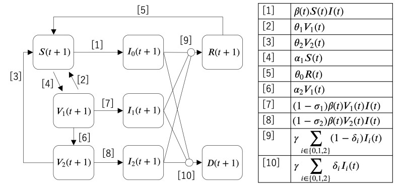
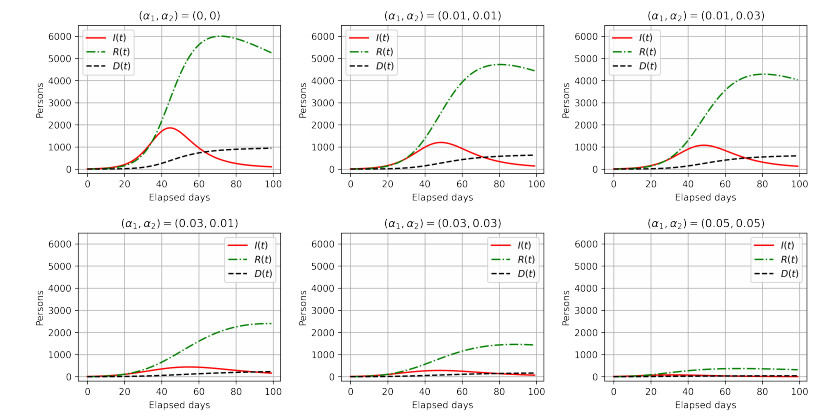
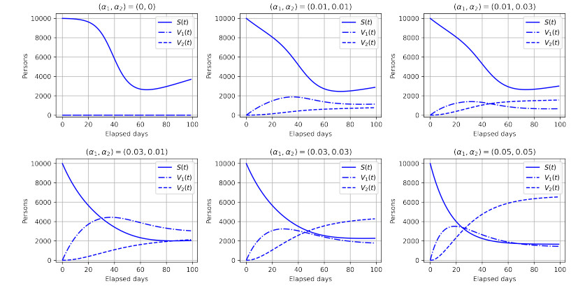
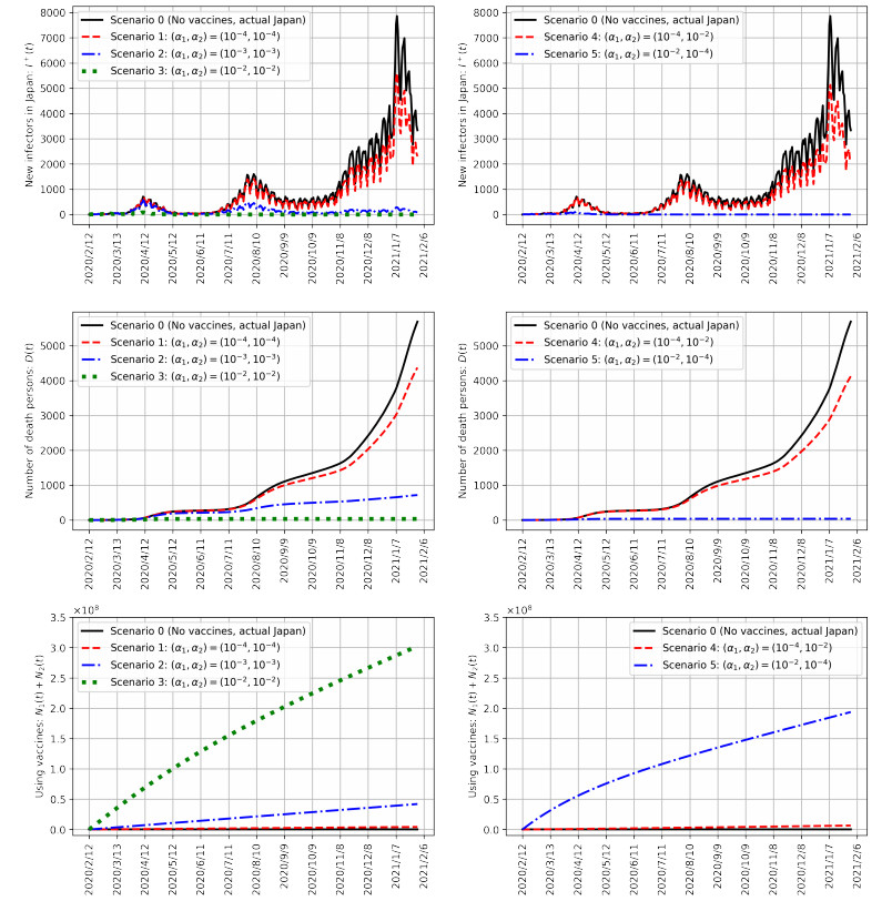
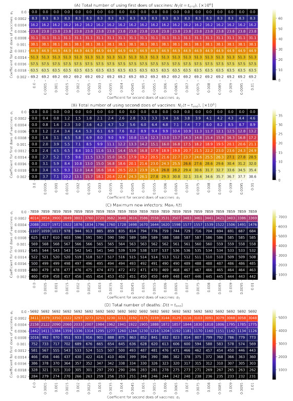
As of August 2021, COVID-19 is still spreading in Japan. Vaccination, one of the key measures to bring COVID-19 under control, began in February 2021. Previous studies have reported that COVID-19 vaccination reduces the number of infections and mortality rates. However, simulations of spreading infection have suggested that vaccination in Japan is insufficient. Therefore, we developed a susceptible–infected–recovered–vaccination1–vaccination2–death model to verify the effect of the first and second vaccination doses on reducing the number of infected individuals in Japan; this includes an infection simulation. The results confirm that appropriate vaccination measures will sufficiently reduce the number of infected individuals and reduce the mortality rate.
Citation: Yuto Omae, Yohei Kakimoto, Makoto Sasaki, Jun Toyotani, Kazuyuki Hara, Yasuhiro Gon, Hirotaka Takahashi. SIRVVD model-based verification of the effect of first and second doses of COVID-19/SARS-CoV-2 vaccination in Japan[J]. Mathematical Biosciences and Engineering, 2022, 19(1): 1026-1040. doi: 10.3934/mbe.2022047
As of August 2021, COVID-19 is still spreading in Japan. Vaccination, one of the key measures to bring COVID-19 under control, began in February 2021. Previous studies have reported that COVID-19 vaccination reduces the number of infections and mortality rates. However, simulations of spreading infection have suggested that vaccination in Japan is insufficient. Therefore, we developed a susceptible–infected–recovered–vaccination1–vaccination2–death model to verify the effect of the first and second vaccination doses on reducing the number of infected individuals in Japan; this includes an infection simulation. The results confirm that appropriate vaccination measures will sufficiently reduce the number of infected individuals and reduce the mortality rate.

| [1] |
G. Buomprisco, S. Ricci, R. Perri, S. De Sio, Health and telework: New challenges after COVID-19 pandemic, Eur. J. Environ. Public Health, 5 (2021), doi: 10.21601/ejeph/9705 doi: 10.21601/ejeph/9705

|
| [2] |
T. Sekizuka, K. Itokawa, K. Yatsu, R. Tanaka, M. Hashino, T. Kawano-Sugaya, et al., COVID-19 genome surveillance at international airport quarantine stations in Japan, J. Travel Med., 28 (2021), doi: 10.1093/jtm/taaa217 doi: 10.1093/jtm/taaa217
|
| [3] |
N. Ahmed, R. A. Michelin, W. Xue, S. Ruj, R. Malaney, S. S. Kanhere, et al., A survey of COVID-19 contact tracing apps, IEEE Access, 8 (2020), 134577–134601, DOI: 10.1109/ACCESS.2020.3010226 doi: 10.1109/ACCESS.2020.3010226
|
| [4] |
P. Supasa, D. Zhou, W. Dejnirattisai, C. Liu, A. J. Mentzer, H. M. Ginn, et al., Reduced neutralization of SARS-CoV-2 B. 1.1. 7 variant by convalescent and vaccine sera, Cell, 184 (2021), 2201–2211, doi: 10.1016/j.cell.2021.02.033 doi: 10.1016/j.cell.2021.02.033
|
| [5] |
C. Liu, H. M. Ginn, W. Dejnirattisai, P. Supasa, B. Wang, A. Tuekprakhon, et al., Reduced neutralization of SARS-CoV-2 B. 1.617 by vaccine and convalescent serum, Cell, 184 (2021), 4220–4236, doi: 10.1016/j.cell.2021.06.020 doi: 10.1016/j.cell.2021.06.020
|
| [6] | J. B. Dunham, An agent-based spatially explicit epidemiological model in MASON, J. Artif. Soc. Social Simul., 9 (2005). |
| [7] |
F. Yang, Q. Yang, X. Liu, P. Wang, SIS evolutionary game model and multi-agent simulation of an infectious disease emergency, Technol. Health Care, 23 (2015), 603–613. doi: 10.3233/THC-150999
|
| [8] |
C. Hou, J. Chen, Y. Zhou, L. Hua, J. Yuan, S. He, et al., The effectiveness of quarantine in Wuhan city against coronavirus disease 2019 (COVID-19): A well-mixed SEIR model analysis, J. Med. Virol., 92 (2020), 841–848, doi: 10.1002/jmv.25827 doi: 10.1002/jmv.25827
|
| [9] |
Z. Liu, P. Magal, G. Webb, Predicting the number of reported and unreported cases of COVID-19 epidemics in China, South Korea, Italy, France, Germany, and the United Kingdom, J. Theor. Biol., 509 (2020), doi: 10.1016/j.jtbi.2020.110501 doi: 10.1016/j.jtbi.2020.110501
|
| [10] |
H. Wang, N. Yamamoto, Using a partial differential equation with Google Mobility data to predict COVID-19 in Arizona, Math. Biosci. Eng., 17 (2020), 4891–4904, doi: 10.3934/mbe.2020266 doi: 10.3934/mbe.2020266
|
| [11] |
I. F. F. dos Santos, G. M. A. Almeida, F. A. B. F. de Moura, Adaptive SIR model for propagation of SARS-CoV-2 in Brazil, Phys. A, 569 (2021), doi: 10.1016/j.physa.2021.125773 doi: 10.1016/j.physa.2021.125773
|
| [12] |
S. Kurahashi, Estimating effectiveness of preventing measures for 2019 novel coronavirus diseases (COVID-19), Trans. Jpn. Soc. Artif. Intell., 35 (2020), D-K28-1, doi: 10.1527/tjsai.D-K28 doi: 10.1527/tjsai.D-K28
|
| [13] |
M. Niwa, Y. Hara, S. Sengoku, K. Kodama, Effectiveness of social measures against COVID-19 outbreaks in several Japanese regions analyzed by system dynamic modeling, SSRN, 3653579 (2020), doi: 10.2139/ssrn.3653579 doi: 10.2139/ssrn.3653579
|
| [14] |
Y. Omae, Y. Kakimoto, J. Toyotani, K. Hara, Y. Gon, H. Takahashi, Impact of removal strategies of stay-at-home orders on the number of COVID-19 infectors and people leaving their homes, Int. J. Innov. Comput. Inf. Control, 17 (2021), 1055–1065, doi: 10.24507/ijicic.17.03.1055 doi: 10.24507/ijicic.17.03.1055
|
| [15] |
Y. Omae, Y. Kakimoto, J. Toyotani, K. Hara, Y. Gon, H. Takahashi, SIR model-based verification of effect of COVID-19 Contact-Confirming Application (COCOA) on reducing infectors in Japan, Math. Biosci. Eng., 18 (2021), 6506–6526, doi: 10.3934/mbe.2021323 doi: 10.3934/mbe.2021323
|
| [16] | G. L. Vasconcelos, A. M. S. Macêdo, G. C. Duarte-Filho, A. A. Brum, R. Ospina, F. A. G. Almeida, Power law behaviour in the saturation regime of fatality curves of the COVID-19 pandemic, Sci. Rep., 11 (2021), article number: 4619, doi: 10.1038/s41598-021-84165-1 |
| [17] | A. M. S. Macêdo, A. A. Brum, G. C. Duarte-Filho, F. A. G. Almeida, R. Ospina, G. L. Vasconcelos, A comparative analysis between a SIRD compartmental model and the Richards growth model, medRxiv, doi: 10.1101/2020.08.04.20168120 |
| [18] |
A. B. Vogel, I. Kanevsky, Y. Che, et al., BNT162b vaccines protect rhesus macaques from SARS-CoV-2, Nature, 592 (2021), 283–289, doi: 10.1038/s41586-021-03275-y doi: 10.1038/s41586-021-03275-y
|
| [19] |
N. Doria-Rose, M. S. Suthar, M. Makowski, S. O'Connell, A. B. McDermott, B. Flach, et al., Antibody persistence through 6 months after the second dose of mRNA-1273 vaccine for Covid-19, N. Engl. J. Med., 384 (2021), 2259–2261, doi: 10.1056/NEJMc2103916 doi: 10.1056/NEJMc2103916
|
| [20] |
M. Scully, D. Singh, R. Lown, A. Poles, T. Solomon, M. Levi, et al., Pathologic antibodies to platelet factor 4 after ChAdOx1 nCoV-19 vaccination, N. Engl. J. Med., 384 (2021), 2202–2211, doi: 10.1056/NEJMoa2105385 doi: 10.1056/NEJMoa2105385
|
| [21] | Ministry of Health, Labour, and Welfare, COVID-19 Vaccine, Available from: https://www.mhlw.go.jp/stf/covid-19/vaccine.html |
| [22] | Government Chief Information Officers' Portal, Japan, Information of COVID-19 vaccine in Japan, Available from: https://cio.go.jp/c19vaccine_dashboard |
| [23] | W. K. Wong, F. H. Juwono, T. H. Chua, Sir simulation of covid-19 pandemic in malaysia: will the vaccination program be effective?, (2021), arXiv preprint arXiv: 2101.07494. https://arXiv.org/abs/2101.07494 |
| [24] |
S. Romero-Brufau, A. Chopra, R. Raskar, J. Subramanian, A. Singh, Y. Dong, et al., Public health impact of delaying second dose of BNT162b2 or mRNA-1273 covid-19 vaccine: Simulation agent based modeling study, Br. Med. J., 373 (2021), doi: 10.1136/bmj.n1087 doi: 10.1136/bmj.n1087
|
| [25] |
J. Li, P. Giabbanelli, Returning to a normal life via COVID-19 vaccines in the United States: a large-scale agent-based simulation study, JMIR Med. Inf., 9 (2021), e27419, doi: 10.2196/27419 doi: 10.2196/27419
|
| [26] | P. Kumar, V. S. Erturk, M. Murillo-Arcila, A new fractional mathematical modelling of COVID-19 with the availability of vaccine, Results Phys., 24 (2021), article number 104213, doi: 10.1016/j.rinp.2021.104213 |
| [27] | R. Ghostine M. Gharamti, S. Hassrouny, I. Hoteit, An extended SEIR model with vaccination for forecasting the COVID-19 pandemic in Saudi Arabia using an ensemble Kalman filter, Mathematics, 9 (2021), article number 636, doi: 10.3390/math9060636 |
| [28] |
R. Rifhat, Z. Teng, C. Wang, Extinction and persistence of a stochastic SIRV epidemic model with nonlinear incidence rate, Adv. Differ. Equ., 200 (2021), doi: 10.1186/s13662-021-03347-3 doi: 10.1186/s13662-021-03347-3
|
| [29] | M. O. Oke, O. M. Ogunmiloro, C. T. Akinwumi, R. A. Raji, Mathematical modeling and stability analysis of a SIRV epidemic model with non-linear force of infection and treatment, Commun. Math. Appl., 10 (2019), 717–731. |
| [30] |
M. Ishikawa, Optimal strategies for vaccination using the stochastic SIRV model, Trans. Inst. Syst. Control Inf. Eng., 25 (2012), 343–348, doi: 10.5687/iscie.25.343 doi: 10.5687/iscie.25.343
|
| [31] |
X. Meng, Z. Cai, H. Dui, H. Cao, Vaccination strategy analysis with SIRV epidemic model based on scale-free networks with tunable clustering, IOP Conf. Ser. Mater. Sci. Eng., 1043 (2021), doi: 10.1088/1757-899X/1043/3/032012 doi: 10.1088/1757-899X/1043/3/032012
|
| [32] |
J. Farooq, M. A. Bazaz, A novel adaptive deep learning model of Covid-19 with focus on mortality reduction strategies, Chaos Soliton. Fract., 138 (2020), doi: 10.1016/j.chaos.2020.110148 doi: 10.1016/j.chaos.2020.110148
|
| [33] |
N. Dagan, N. Barda, E. Kepten, O. Miron, S. Perchik, M. A. Katz, et al., BNT162b2 mRNA Covid-19 vaccine in a nationwide mass vaccination setting, N. Engl. J. Med., 384 (2021), 1412–1423, doi: 10.1056/NEJMoa2101765 doi: 10.1056/NEJMoa2101765
|
| [34] |
M. Lounis, D. K. Bagal, Estimation of SIR model's parameters of COVID-19 in Algeria, Bull. Nat. Res. Centre, 44 (2020), 1–6, doi: 10.1186/s42269-020-00434-5 doi: 10.1186/s42269-020-00434-5
|
| [35] |
X. Geng, G. G. Katul, F. Gerges, E. Bou-Zeid, H. Nassif, M. C. Boufadel, A kernel-modulated SIR model for Covid-19 contagious spread from county to continent, Proc. Nat. Acad. Sci., 118 (2021), doi: 10.1073/pnas.2023321118 doi: 10.1073/pnas.2023321118
|
| [36] | Ministry of Health, Labour, and Welfare, Open data of positive result of COVID-19, (2021), Available from: https://www.mhlw.go.jp/content/pcr_positive_daily.csv |
| [37] |
G. Kobayashi, S. Sugasawa, H. Tamae, T. Ozu, Predicting intervention effect for COVID-19 in Japan: State space modeling approach, Biosci. Trends, 14 (2020), 174–181, doi: 10.5582/bst.2020.03133 doi: 10.5582/bst.2020.03133
|
| [38] |
J. M. Dan, J. Mateus, Y. Kato, K. M. Hastie, E. D. Yu, C. E. Faliti, et al., Immunological memory to SARS-CoV-2 assessed for up to 8 months after infection, Science, 371 (2021), doi: 10.1126/science.abf4063 doi: 10.1126/science.abf4063
|
| [39] |
J. Lopez Bernal, N. Andrews, C. Gower, E. Gallagher, R. Simmons, S. Thelwall, et al., Effectiveness of Covid-19 vaccines against the B. 1.617. 2 (delta) variant, N. Engl. J. Med., (2021), doi: 10.1056/NEJMoa2108891 doi: 10.1056/NEJMoa2108891
|
| [40] | The 44th Novel Coronavirus Expert Meeting (21 July 2021), Document 2–4, Available from: https://www.mhlw.go.jp/content/10900000/000809571.pdf |
| [41] | Johns Hopkins University, COVID-19 data repository by the center for systems science and engineering (CSSE) at Johns Hopkins University, Available from: https://github.com/CSSEGISandData/COVID-19 |
Figures(6) / Tables(1)

Yuto Omae, Yohei Kakimoto, Makoto Sasaki, Jun Toyotani, Kazuyuki Hara, Yasuhiro Gon, Hirotaka Takahashi. SIRVVD model-based verification of the effect of first and second doses of COVID-19/SARS-CoV-2 vaccination in Japan[J]. Mathematical Biosciences and Engineering, 2022, 19(1): 1026-1040. doi: 10.3934/mbe.2022047


 DownLoad: