On three dimensional fractal dynamics with fractional inputs and applications

Emile Franc Doungmo Goufo; Abdon Atangana; Emile Franc Doungmo Goufo; Abdon Atangana

doi:10.3934/math.2022114

AIMS Mathematics

2022, Volume 7, Issue 2: 1982-2000. doi: 10.3934/math.2022114

Previous Article Next Article

Research article Special Issues

On three dimensional fractal dynamics with fractional inputs and applications

Emile Franc Doungmo Goufo ^{1
,
,},
Abdon Atangana ²

1.
Department of Mathematical Sciences, University of South Africa, Florida 0003, South Africa
2.
Institute for Groundwater Studies, University of the Free State, Bloemfontein 9300, South Africa

Received: 19 August 2021 Accepted: 24 October 2021 Published: 05 November 2021
MSC : 65P20, 65P30, 28A80, 65J15, 26A33

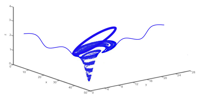
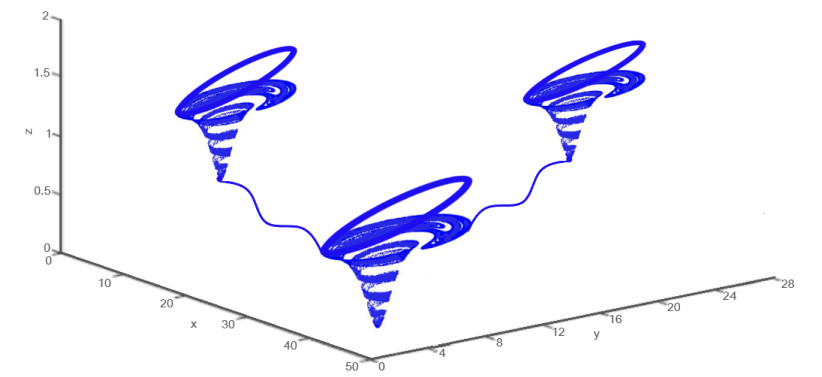
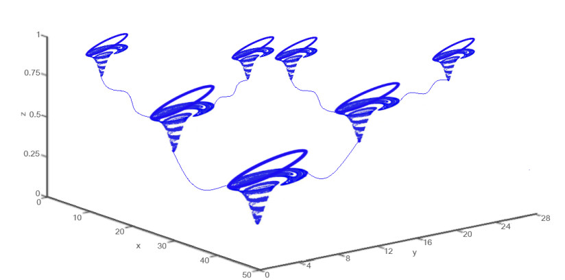
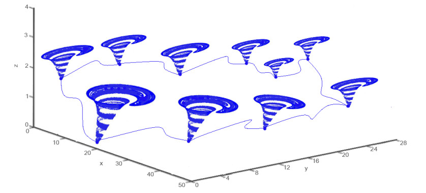
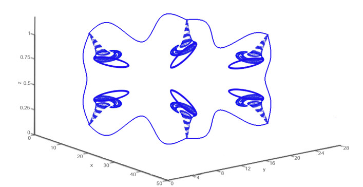
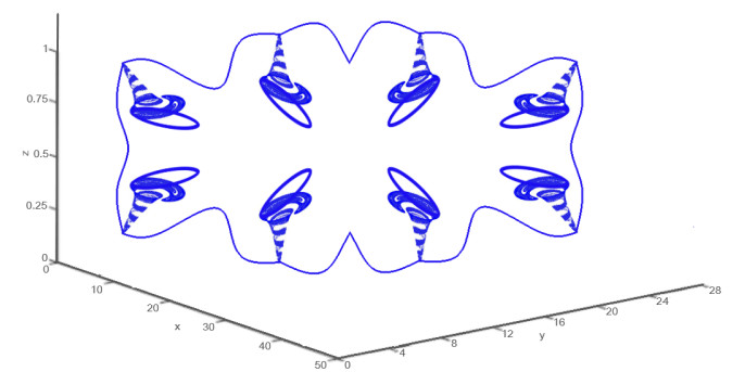
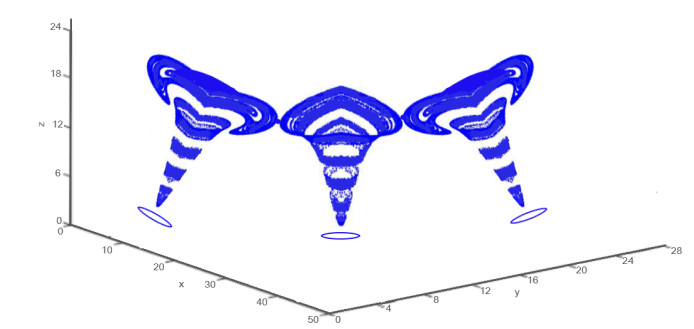
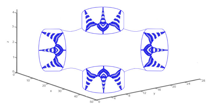
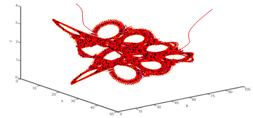
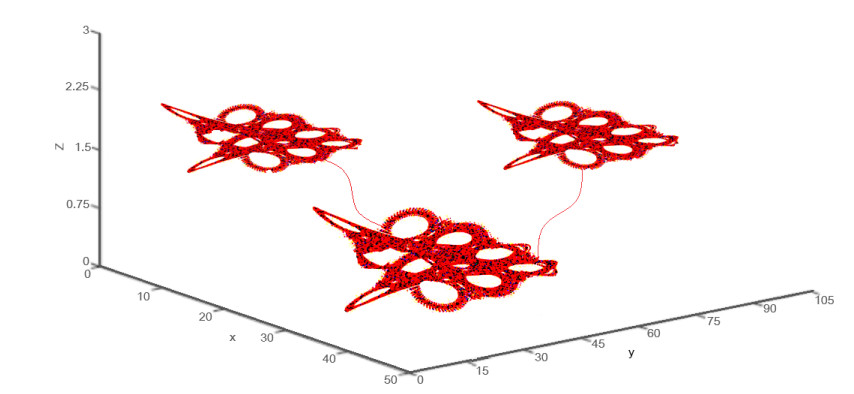
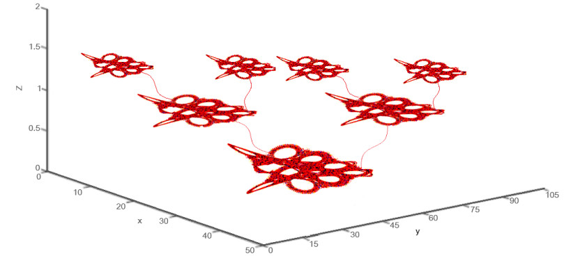
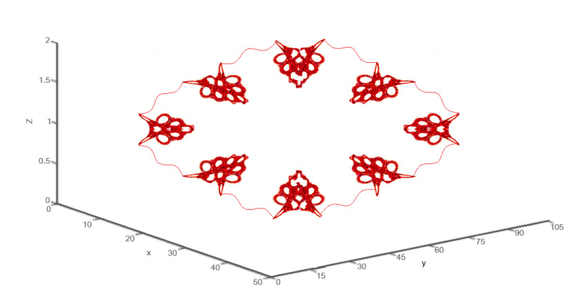
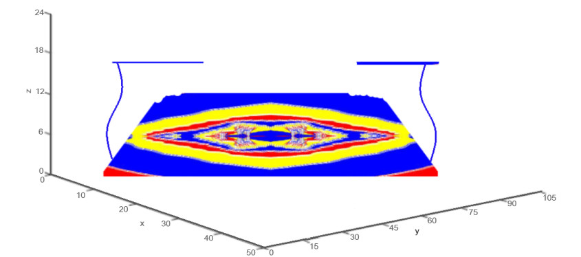
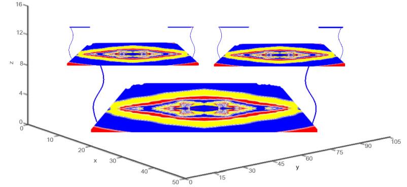
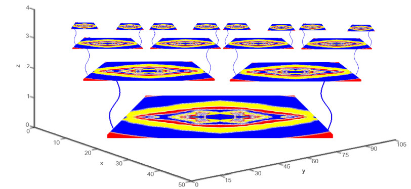
The environment around us naturally represents number of its components in fractal structures. Some fractal patterns are also artificially simulated using real life mathematical systems. In this paper, we use the fractal operator combined to the fractional operator with both exponential and Mittag-leffler laws to analyze and solve generalized three-dimensional systems related to real life phenomena. Numerical solutions are provided in each case and applications to some related systems are given. Numerical simulations show the existence of the models' initial three-dimensional structure followed by its self- replication in fractal structure mathematically produced. The whole dynamics are also impacted by the fractional part of the operator as the derivative order changes.

Keywords:

Citation: Emile Franc Doungmo Goufo, Abdon Atangana. On three dimensional fractal dynamics with fractional inputs and applications[J]. AIMS Mathematics, 2022, 7(2): 1982-2000. doi: 10.3934/math.2022114

Related Papers:

[1]	Khaled M. Saad, Manal Alqhtani . Numerical simulation of the fractal-fractional reaction diffusion equations with general nonlinear. AIMS Mathematics, 2021, 6(4): 3788-3804. doi: 10.3934/math.2021225
[2]	Nadiyah Hussain Alharthi, Abdon Atangana, Badr S. Alkahtani . Numerical analysis of some partial differential equations with fractal-fractional derivative. AIMS Mathematics, 2023, 8(1): 2240-2256. doi: 10.3934/math.2023116
[3]	Abdon Atangana, Ali Akgül . Analysis of a derivative with two variable orders. AIMS Mathematics, 2022, 7(5): 7274-7293. doi: 10.3934/math.2022406
[4]	Hasib Khan, Jehad Alzabut, Anwar Shah, Sina Etemad, Shahram Rezapour, Choonkil Park . A study on the fractal-fractional tobacco smoking model. AIMS Mathematics, 2022, 7(8): 13887-13909. doi: 10.3934/math.2022767
[5]	Amir Ali, Abid Ullah Khan, Obaid Algahtani, Sayed Saifullah . Semi-analytical and numerical computation of fractal-fractional sine-Gordon equation with non-singular kernels. AIMS Mathematics, 2022, 7(8): 14975-14990. doi: 10.3934/math.2022820
[6]	Ihtisham Ul Haq, Shabir Ahmad, Sayed Saifullah, Kamsing Nonlaopon, Ali Akgül . Analysis of fractal fractional Lorenz type and financial chaotic systems with exponential decay kernels. AIMS Mathematics, 2022, 7(10): 18809-18823. doi: 10.3934/math.20221035
[7]	Muhammad Farman, Ali Akgül, Kottakkaran Sooppy Nisar, Dilshad Ahmad, Aqeel Ahmad, Sarfaraz Kamangar, C Ahamed Saleel . Epidemiological analysis of fractional order COVID-19 model with Mittag-Leffler kernel. AIMS Mathematics, 2022, 7(1): 756-783. doi: 10.3934/math.2022046
[8]	Abdon Atangana, Seda İğret Araz . Extension of Chaplygin's existence and uniqueness method for fractal-fractional nonlinear differential equations. AIMS Mathematics, 2024, 9(3): 5763-5793. doi: 10.3934/math.2024280
[9]	Rahat Zarin, Amir Khan, Pushpendra Kumar, Usa Wannasingha Humphries . Fractional-order dynamics of Chagas-HIV epidemic model with different fractional operators. AIMS Mathematics, 2022, 7(10): 18897-18924. doi: 10.3934/math.20221041
[10]	Muhammad Farman, Aqeel Ahmad, Ali Akgül, Muhammad Umer Saleem, Kottakkaran Sooppy Nisar, Velusamy Vijayakumar . Dynamical behavior of tumor-immune system with fractal-fractional operator. AIMS Mathematics, 2022, 7(5): 8751-8773. doi: 10.3934/math.2022489

Abstract

1. Introduction

The world within which humans leave is very complex and can exhibit many different behavior. Some of these behaviors are very difficult to be analyzed via observation only. However, some can be replicate using mathematical formulas. Mathematicians have classified some real world behaviors as they were able to replicate those using mathematical formulas. In the literature, one will find, concepts like fractal, chaos, random walk, Levy flight motions ^[1], Brownian motions ^[2], Bernoulli process, Markovian process ^[3], non-Markovian process ^[4] and many other that will not be listed here. The concept of fractal have attracted attention of researchers from all background due to their appearance in real world ^[5,6,7,8,9]. It is even believed that, this concept was already developed in Africas cultures as many of their constructions resembled self-similarities, for example, the structure of their traditional kingdom resembled the structure of the villages. It has also mentioned that, their traditional clothes could be seeing as fractal designs. The concept has been developed in mathematics, for example some mathematical mapping have been used to replicate these fractal behaviors observed in real world problems. Some of the well-known mapping are the Julia, Mandelbrot, Fatou and Newton mappings. These mapping have been intensively studies as they are able to produce many different type of theoretical fractal behaviors. In particular these mapping are derived using polynomials with two dimensional complex numbers. The concept was extended in system call quaternion which is a 4 dimensional complex numbers. However, Atangana and Toufik argued that the nature within which humans leave is neither two dimensional nor 4 dimensional therefore fractal represented by these two sets may not be very representative in humans world therefore they suggested a set 3-dimensional complex numbers and called it Trinition ^[10]. The Trinition polynomial are able to reproduce fractal in 3-dimension which can be found in many real world problems. Above this concept of mapping, mathematicians have suggested other operators called fractal differentiation and integration, these mathematical operators are able to depict some degree of self-similarities. Recall that many authors have applied the concept of fractal-fractional operator in number of mathematical circumstances and proposed many related applications in connection to real life phenomena. Some of them are found in ^{[11,12,13,14]}. Some researchers have applied the concept of fractal-fractional in various processes related to real life phenomena, such as mathematical epidemiology, control theory, Levy statistics continuous time random walk, biomedical engineering, fractional signal and image processing, fractional filters motion and nonlocal phenomena ^{[8,11,15,16,17,18]}. We can also mention the concept of self-similarity found in the nature around us which takes into account the fractal dimension applicable in the domain of engineering and including aspects like fatigue loading conditions and fracture surface analysis ^[19]. The authors in ^[20] pointed out the fractal impact on microstructure and its relationship to properties such as fracture toughness or fracture energy. The variety of these works and publications show the vast range and scope that cover the application of fractional processes combined with fractal dynamics in various domains of sciences. In this paper, we shall analyze some real world problems using fractal-fractional differential operators.

2. Preliminaries on fractal-fractional derivatives

The concept of fractal-fractional derivative was developed and introduced recently with the aim of attracting and describing a considerable amount of non-local problems found in nature and also respecting the fractal structure that characterize them ^[11,13,15]. It is defined to be the convolution of fractal differential operator with the usual functions (power, exponential and Mittag-Leffler laws) of fractional calculus. The literature comprises various definitions of the fractal-fractional derivative depending on the type of law used. Some are given as follow:

Definition 2.1. We consider $X\in \mathbb{R}^3$ , $a, b\in \mathbb{R},$ and assume that $h(t, \mathbf{x})$ defined on $(a, b)\times X$ is $t-$ fractal differentiable with the order $\gamma$ on the interval $(a, b)$ then, the fractal-fractional derivative of $h$ of order $\gamma$ in the sense of Riemann-Liouville with power law reads as:

$\begin{equation} ^{FRp}D^\gamma_{t}h(t, \mathbf{x}) = \frac{1}{\Gamma\left(1-\gamma \right)}\frac{\partial}{\partial t^\gamma}\int^t_0h\left(\vartheta, \mathbf{x}\right)(t-\vartheta)^{-\gamma}d\vartheta, \end{equation}$

(2.1)

where $\frac{\partial}{\partial t^\gamma}h$ is defined as

$\frac{\partial}{\partial t^\gamma}h(t_0, \mathbf{x}) = \lim\limits_{t \to t_0}\frac{h(t, \mathbf{x})-h(t_0, \mathbf{x})}{t^\gamma- t_0^\gamma}.$

The generalized version of (2.1) is defined by

$\begin{equation} ^{FRp}D^{\gamma, \varsigma}_{t}h(t, \mathbf{x}) = \frac{1}{\Gamma\left(1-\gamma \right)}\frac{\partial^\varsigma}{\partial t^\gamma}\int^t_0h\left(\vartheta, \mathbf{x}\right)(t-\vartheta)^{-\gamma}d\vartheta, \end{equation}$

(2.2)

with $\varsigma > 0$ and $\frac{\partial^\varsigma}{\partial t^\gamma}h$ given by

$\frac{\partial^\varsigma}{\partial t^\gamma}h(t_0, \mathbf{x}) = \lim\limits_{t \to t_0}\frac{h^\varsigma(t, \mathbf{x})-h^\varsigma(t_0, \mathbf{x})}{t^\gamma- t_0^\gamma}.$

Similarly, the Caputo version od that definition can be given:

Definition 2.2. We consider $X\in \mathbb{R}^3$ , $a, b\in \mathbb{R},$ and assume that $h(t, \mathbf{x})$ defined on $(a, b)\times X$ is $t-$ fractal differentiable with the order $\gamma$ on the interval $(a, b)$ then, the fractal-fractional derivative of $h$ of order $\gamma$ in the sense of Caputo with power law reads as:

$\begin{equation} ^{FCp}D^\gamma_{t}h(t, \mathbf{x}) = \frac{1}{\Gamma\left(1-\gamma \right)}\int^t_0\frac{\partial}{\partial \vartheta^\gamma }h\left(\vartheta, \mathbf{x}\right)(t-\vartheta)^{-\gamma}d\vartheta, \end{equation}$

(2.3)

with the generalized version

$\begin{equation} ^{FCp}D^{\gamma, \varsigma}_{t}h(t, \mathbf{x}) = \frac{1}{\Gamma\left(1-\gamma \right)}\int^t_0\frac{\partial^\varsigma}{\partial \vartheta^\gamma}h\left(\vartheta, \mathbf{x}\right)(t-\vartheta)^{-\gamma}d\vartheta. \end{equation}$

(2.4)

The following definitions are related to exponential law:

Definition 2.3. We consider $X\in \mathbb{R}^3$ , $a, b\in \mathbb{R},$ and assume that $h(t, \mathbf{x})$ defined on $(a, b)\times X$ is $t-$ fractal differentiable with the order $\gamma$ on the interval $(a, b)$ then, the fractal-fractional derivative of $h$ of order $\gamma$ in the sense of Riemann-Liouville with exponential law reads as:

$\begin{equation} ^{FRe}D^\gamma_{t}h(t, \mathbf{x}) = \frac{\boldsymbol{q}(\gamma)}{\left(1-\gamma \right)}\frac{\partial}{\partial t^\gamma}\int^t_0h\left(\vartheta, \mathbf{x}\right)\exp \left( { \frac{-\gamma (t-\vartheta)}{1-\gamma} } \right) d\vartheta, \end{equation}$

(2.5)

where $\boldsymbol{q}(0) = \boldsymbol{q}(1) = 1$ with the generalized version

$\begin{equation} ^{FRe}D^{\gamma, \varsigma}_{t}h(t, \mathbf{x}) = \frac{\boldsymbol{q}(\gamma)}{\left(1-\gamma \right)}\frac{\partial^\varsigma}{\partial t^\gamma}\int^t_0h\left(\vartheta, \mathbf{x}\right)\exp \left( { \frac{-\gamma (t-\vartheta)}{1-\gamma} } \right) d\vartheta. \end{equation}$

(2.6)

Definition 2.4. We consider $X\in \mathbb{R}^3$ , $a, b\in \mathbb{R},$ and assume that $h(t, \mathbf{x})$ defined on $(a, b)\times X$ is $t-$ fractal differentiable with the order $\gamma$ on the interval $(a, b)$ then, the fractal-fractional derivative of $h$ of order $\gamma$ in the sense of Caputo with exponential law reads as:

$\begin{equation} ^{FCe}D^\gamma_{t}h(t, \mathbf{x}) = \frac{\boldsymbol{q}(\gamma)}{\left(1-\gamma \right)}\int^t_0\frac{\partial}{\partial \vartheta^\gamma}h\left(\vartheta, \mathbf{x}\right)\exp \left( { \frac{-\gamma (t-\vartheta)}{1-\gamma} } \right) d\vartheta, \end{equation}$

(2.7)

with the generalized version

$\begin{equation} ^{FCe}D^{\gamma, \varsigma}_{t}h(t, \mathbf{x}) = \frac{\boldsymbol{q}(\gamma)}{\left(1-\gamma \right)}\int^t_0\frac{\partial^\varsigma}{\partial \vartheta^\gamma}h\left(\vartheta, \mathbf{x}\right)\exp \left( { \frac{-\gamma (t-\vartheta)}{1-\gamma} } \right) d\vartheta. \end{equation}$

(2.8)

The following definitions are related to Mittag-Leffler law:

Definition 2.5. We consider $X\in \mathbb{R}^3$ , $a, b\in \mathbb{R},$ and assume that $h(t, \mathbf{x})$ defined on $(a, b)\times X$ is $t-$ fractal differentiable with the order $\gamma$ on the interval $(a, b)$ then, the fractal-fractional derivative of $h$ of order $\gamma$ in the sense of Riemann-Liouville with Mittag-Leffler law reads as:

$\begin{equation} ^{FRm}D^{\gamma}_{t}h(t, \mathbf{x}) = \frac{\boldsymbol{w}(\gamma)}{\left(1-\gamma \right)}\frac{\partial}{\partial t^\gamma}\int^t_0h\left(\vartheta, \mathbf{x}\right)E_\gamma \left( { \frac{-\gamma (t-\vartheta)^\gamma}{1-\gamma} } \right) d\vartheta, \end{equation}$

(2.9)

where $\boldsymbol{w}(\gamma)$ is a regularization function. Here the generalized version

$\begin{equation} ^{FRm}D^{\gamma, \varsigma}_{t}h(t, \mathbf{x}) = \frac{\boldsymbol{w}(\gamma)}{\left(1-\gamma \right)}\frac{\partial^\varsigma}{\partial t^\gamma}\int^t_0h\left(\vartheta, \mathbf{x}\right)E_\gamma \left( { \frac{-\gamma (t-\vartheta)^\gamma}{1-\gamma} } \right) d\vartheta. \end{equation}$

(2.10)

Definition 2.6. We consider $X\in \mathbb{R}^3$ , $a, b\in \mathbb{R},$ and assume that $h(t, \mathbf{x})$ defined on $(a, b)\times X$ is $t-$ fractal differentiable with the order $\gamma$ on the interval $(a, b)$ then, the fractal-fractional derivative of $h$ of order $\gamma$ in the sense of Caputo with Mittag-Leffler law reads as:

$\begin{equation} ^{FCm}D^{\gamma}_{t}h(t, \mathbf{x}) = \frac{\boldsymbol{w}(\gamma)}{\left(1-\gamma \right)}\int^t_0\frac{\partial}{\partial \vartheta^\gamma}h\left(\vartheta, \mathbf{x}\right)E_\gamma \left( { \frac{-\gamma (t-\vartheta)^\gamma}{1-\gamma} } \right) d\vartheta, \end{equation}$

(2.11)

where $\boldsymbol{w}(\gamma)$ is a regularization real function related to the definition and with a more general version given as

$\begin{equation} ^{FCm}D^{\gamma, \varsigma}_{t}h(t, \mathbf{x}) = \frac{\boldsymbol{w}(\gamma)}{\left(1-\gamma \right)}\int^t_0\frac{\partial^\varsigma}{\partial \vartheta^\gamma}h\left(\vartheta, \mathbf{x}\right)E_\gamma \left( { \frac{-\gamma (t-\vartheta)^\gamma}{1-\gamma} } \right) d\vartheta. \end{equation}$

(2.12)

3. Numerical solution with the definition in Caputo sense with exponential law

We use the Definition 2.2 formulated in the previous section and express the numerical solution for the fractal-fractional differential equations using the predictor-correction method. This scheme was suggested very recently to help recover some missing terms the scheme suggested by Atangana and Seda ^[21]. Hence, we consider a general non-linear equation with fractal-fractional differential operator given as

$\begin{eqnarray} \left\{\begin{array}{llll} {^{FRe}D^\gamma_t}Y(t) = f(t, Y(t)), &&\\ Y(0) = Y_0. \end{array}\right. \end{eqnarray}$

(3.1)

To proceed we convert the equation into Volterra version as

$Y(t) = Y(0)+\frac{\beta}{\Gamma(\gamma)}\int_0^t \tau^{1-\beta}f(\tau, Y(\tau))(t-\tau)^{\gamma-1}d\tau.$

For simplicity, we set $\tau^{1-\beta}f(\tau, Y(\tau)) = F(\tau, Y(\tau)).$ Following the result by ^[22], we have

$\begin{equation} \begin{aligned} Y_{n+1}& = Y_0+\delta_{n+1}+\frac{(\Delta t)^\gamma}{\Gamma(\gamma+1)}F(t_0, Y_0)[(n+1)^\gamma-n^\gamma]\\ &+\frac{(\Delta t)^\gamma}{\Gamma(\gamma+2)}[F(t_1, Y_1)-F(t_0, Y_0)][(n+1)^{\gamma+1}-n^{\gamma+1}-(\gamma+1)n^\gamma]\\ &+\frac{(\Delta t)^\gamma}{\Gamma(\gamma+1)}F(t_{n+1}, Y_{n+1}^p)+\frac{\gamma(\Delta t)^\gamma}{\Gamma(\gamma+2)} \left( { F(t_{n}, Y_{n})-F(t_{n+1}, Y_{n+1}^p) } \right) \\ &-\frac{\gamma(\Delta t)^\gamma}{2\Gamma(\gamma+3)} \left( { F(t_{n+1}, Y_{n+1}^p)-2F(t_{n}, Y_{n}) } \right) +F(t_{n-1}, Y_{n-1}), \end{aligned} \end{equation}$

(3.2)

where the predictor is given as

$\begin{equation} \begin{aligned} Y_{n+1}^p& = Y_0+\frac{(\Delta t)^\gamma}{\Gamma(\gamma+1)} \sum\limits_{k = 0}^{1}F(t_k, Y_k)[(n-k+1)^\gamma-(n-k)^\gamma]\\ &+\frac{(\Delta t)^\gamma}{\Gamma(\gamma+2)}\sum\limits_{k = 0}^{1}[F(t_{k+1}, Y_{k+1})-F(t_k, Y_k)]\left[(n-k+1)^{\gamma+1}\right.\\ &\left.-(n-k)^{\gamma+1}-(\gamma+1)(n-k)^\gamma\right]\\ &+\frac{(\Delta t)^\gamma}{\Gamma(\gamma+1)}\sum\limits_{k = 2}^{n}F(t_{k-2}, Y_{k-2})[(n-k+1)^{\gamma}-(n-k)^{\gamma}]\\ &+\frac{(\Delta t)^\gamma}{\Gamma(\gamma+2)}\sum\limits_{k = 2}^{n}[F(t_{k-1}, Y_{k-1})-F(t_{k-2}, Y_{k-2})]\left[(n-k+1)^{\gamma}(n-k+3+2\gamma)\right.\\ &\left.-(n-k)^\gamma (n-k+3+3\gamma)\right]\\ &+\frac{(\Delta t)^\gamma}{2\Gamma(\gamma+3)}\sum\limits_{k = 2}^{n}[F(t_{k}, Y_{k})-2F(t_{k-1}, Y_{k-1})+F(t_{k-2}, Y_{k-2})]\left[(n-k+1)^{\gamma}\left(2(n-j)^2\right.\right.\\ &\left.\left.+(3\gamma +10)(n-k)+2\gamma^2+9\gamma+12\right)-(n-k)^\gamma\left(2(n-k)^2\right.\right.\\ &\left.\left.+(5\gamma+10)(n-k)+6\gamma^2+18\gamma+12\right)\right].\\ \end{aligned} \end{equation}$

(3.3)

Finally

$\begin{equation} \begin{aligned} \delta_{n}& = \frac{(\Delta t)^\gamma}{\Gamma(\gamma+1)} \sum\limits_{k = 1}^{n}\left[F(t_{k+1}, Y_{k+1})[(n-k+1)^\gamma-(n-k)^\gamma]\right.\\ &+\frac{(\Delta t)^\gamma}{\Gamma(\gamma+2)}\sum\limits_{k = 1}^{n}[F(t_{k+1}, Y_{k+1})-F(t_k, Y_k)][(n-k+\gamma)(n-k+1)^{\gamma}-(n-k)^{\gamma+1}]\\ &+\frac{(\Delta t)^\gamma}{2\Gamma(\gamma+3)}\sum\limits_{k = 1}^{n} \left( { F(t_{k+1}, Y_{k+1})-2F(t_{k}, Y_{k})+F(t_{k-1}, Y_{k-1}) } \right) \left[(n-k+1)^{\gamma}\left(2(n-k)^2\right.\right.\\ &\left.\left.-\gamma(n-k+1)+2(n-k)\right)-(n-k)^{\gamma}(2(n-k)^2-\gamma(n-k)+2(n-k))\right]. \end{aligned} \end{equation}$

(3.4)

4. Numerical solution with the definition in Atangana-Baleanu sense with Mittag-Leffler law

Using the Definition 2.5, we consider a general non-linear equation with fractal-fractional differential operator given as

$\begin{eqnarray} \left\{\begin{array}{llll} {^{FRm}D^\gamma_t}Y(t) = f(t, Y(t)), &&\\ Y(0) = Y_0 \end{array}\right. \end{eqnarray}$

(4.1)

Following the same approach, we convert the equation into Volterra version as

$Y(t) = Y(0)+\frac{\beta \gamma}{W(\gamma)\Gamma(\gamma)}\int_0^t \tau^{1-\beta}f(\tau, Y(\tau))(t-\tau)^{\gamma-1}d\tau+\frac{1-\gamma}{W(\gamma)}f(t, Y(t)).$

Taking again $\tau^{1-\beta}f(\tau, Y(\tau)) = F(\tau, Y(\tau)),$ we obtain

$Y_{n+1} = Y_0+\frac{\gamma}{W(\gamma)} \delta_{n+1}+\frac{(\Delta t)^\gamma}{\Gamma(\gamma+1)}F(t_0, Y_0)[(n+1)^\gamma-n^\gamma] \\ +\frac{\gamma}{W(\gamma)}\frac{(\Delta t)^\gamma}{\Gamma(\gamma+2)}[F(t_1, Y_1)-F(t_0, Y_0)][(n+1)^{\gamma+1}-n^{\gamma+1}-(\gamma+1)n^\gamma]\\ +\frac{\gamma}{W(\gamma)} \frac{(\Delta t)^\gamma}{\Gamma(\gamma+1)}F(t_{n+1}, Y_{n+1}^p)+\frac{\gamma(\Delta t)^\gamma}{\Gamma(\gamma+2)} \left( { F(t_{n}, Y_{n})-F(t_{n+1}, Y_{n+1}^p) } \right) \\ -\frac{\gamma}{W(\gamma)}\frac{\gamma(\Delta t)^\gamma}{2\Gamma(\gamma+3)} \left( { F(t_{n+1}, Y_{n+1}^p)-2F(t_{n}, Y_{n}) } \right) +F(t_{n-1}, Y_{n-1})\\ +\frac{1-\gamma}{W(\gamma)}\frac{F(t_n, Y_n)}{t^{1-\beta}},$

(4.2)

where the predictor is given as

$\begin{aligned} Y_{n+1}^{p} & = Y_{0}+\frac{\gamma}{W(\gamma)} \frac{(\Delta t)^{\gamma}}{\Gamma(\gamma+1)} \sum\limits_{k = 0}^{1} F\left(t_{k}, Y_{k}\right)\left[(n-k+1)^{\gamma}-(n-k)^{\gamma}\right] \\ &+\frac{\gamma}{W(\gamma)} \frac{(\Delta t)^{\gamma}}{\Gamma(\gamma+2)} \sum\limits_{k = 0}^{1}\left[F\left(t_{k+1}, Y_{k+1}\right)-F\left(t_{k}, Y_{k}\right)\right]\left[(n-k+1)^{\gamma+1}\right.\\ &\left.-(n-k)^{\gamma+1}-(\gamma+1)(n-k)^{\gamma}\right] \\ &+\frac{\gamma}{W(\gamma)} \frac{(\Delta t)^{\gamma}}{\Gamma(\gamma+1)} \sum\limits_{k = 2}^{n} F\left(t_{k-2}, Y_{k-2}\right)\left[(n-k+1)^{\gamma}-(n-k)^{\gamma}\right] \\ &+\frac{\gamma}{W(\gamma)} \frac{(\Delta t)^{\gamma}}{\Gamma(\gamma+2)} \sum\limits_{k = 2}^{n}\left[F\left(t_{k-1}, Y_{k-1}\right)-F\left(t_{k-2}, Y_{k-2}\right)\right]\left[(n-k+1)^{\gamma}(n-k+3+2 \gamma)\right.\\ &\left.-(n-k)^{\gamma}(n-k+3+3 \gamma)\right] \\ &+\frac{\gamma}{W(\gamma)} \frac{(\Delta t)^{\gamma}}{2 \Gamma(\gamma+3)} \sum\limits_{k = 2}^{n}\left[F\left(t_{k}, Y_{k}\right)-2 F\left(t_{k-1}, Y_{k-1}\right)\right.\\ &\left.+F\left(t_{k-2}, Y_{k-2}\right)\right]\left[( n - k + 1 ) ^ { \gamma } \left(2(n-j)^{2}\right.\right.\\ &\left.+(3 \gamma+10)(n-k)+2 \gamma^{2}+9 \gamma+12\right)-(n-k)^{\gamma}\left(2(n-k)^{2}\right.\\ &\left.\left.+(5 \gamma+10)(n-k)+6 \gamma^{2}+18 \gamma+12\right)\right]+\frac{1-\gamma}{W(\gamma)} \frac{F\left(t_{n}, Y_{n}\right)}{t^{1-\beta}} \end{aligned}$

(4.3)

Finally

$\begin{equation} \begin{aligned} \delta_{n}& = \frac{\gamma}{W(\gamma)}\frac{(\Delta t)^\gamma}{\Gamma(\gamma+1)} \sum\limits_{k = 1}^{n}\left[F(t_{k+1}, Y_{k+1})[(n-k+1)^\gamma-(n-k)^\gamma]\right.\\ &+\frac{\gamma}{W(\gamma)}\frac{(\Delta t)^\gamma}{\Gamma(\gamma+2)}\sum\limits_{k = 1}^{n}[F(t_{k+1}, Y_{k+1})-F(t_k, Y_k)][(n-k+\gamma)(n-k+1)^{\gamma}-(n-k)^{\gamma+1}]\\ &+\frac{\gamma}{W(\gamma)}\frac{(\Delta t)^\gamma}{2\Gamma(\gamma+3)}\sum\limits_{k = 1}^{n} \left( { F(t_{k+1}, Y_{k+1})-2F(t_{k}, Y_{k})+F(t_{k-1}, Y_{k-1}) } \right) \left[(n-k+1)^{\gamma}\left(2(n-k)^2\right.\right.\\ &\left.\left.-\gamma(n-k+1)+2(n-k)\right)-(n-k)^{\gamma}(2(n-k)^2-\gamma(n-k)+2(n-k))\right]+\frac{1-\gamma}{W(\gamma)}\frac{F(t_n, Y_n)}{t^{1-\beta}}. \end{aligned} \end{equation}$

(4.4)

5. Application to some real life phenomena

We use the schemes proposed in the previous section to solve some nature related models and access their behavior when they are under the influence of the fractal fractional operator.

5.1. Application 1: The three-dimentional fractal in tornado system

On the system, we analyze and assess here, the impact of the fractal-fractional derivative in Riemann-Liouville sense with exponential law given in Definition 2.3. To that effect, we combine it with the three-dimensional tornado system proposed in [10,(42)] to get:

$\begin{eqnarray} \left\{\begin{array}{llll} {^{FRe}D^\gamma_t}x(t) = C-\frac{d}{x^2+y^2+r^2}, &&\\ {^{FRe}D^\gamma_t}y(t) = a+b(x\cos z +y \sin z), &&\\ {^{FRe}D^\gamma_t}z(t) = z^2-b(x\sin z - y \cos z), &&\\ \end{array}\right. \end{eqnarray}$

(5.1)

and

$\begin{eqnarray} \left\{\begin{array}{llll} ^{FRe}D^{\gamma, \varsigma}_{t}x(t) = C-\frac{d}{x^2+y^2+r^2}, &&\\ ^{FRe}D^{\gamma, \varsigma}_{t}y(t) = a+b(x\cos z +y \sin z), &&\\ ^{FRe}D^{\gamma, \varsigma}_{t}z(t) = z^2-b(x\sin z - y \cos z).&&\\ \end{array}\right. \end{eqnarray}$

(5.2)

In order to conveniently solve the combined fractional and fractal system, it is important to associate it with the following initial conditions:

$\begin{equation} x(0) = \tilde{x}(x), \ y(0) = \tilde{y}(y), \ z(0) = \tilde{z}(z). \end{equation}$

(5.3)

Numerical simulations of model (5.1) and (5.3) are shown in Figure 1 to Figure 6 which show the three-dimensional fractal structures to be in a self-replication process with the influence of the fractional derivative that extends the self-replication in number and shape as the derivative order varies. Similar behavior is produced and observed for the model (5.2) and (5.3) as shown in Figure 7 and Figure 8.

Figure 1. The tornado system representing the model (5.1) and (5.3) for

$\gamma = 0.9$ and

$x(0) = \tilde{x}(x) = 0.2, \ y(0) = \tilde{y}(y) = 0.02, \ z(0) = \tilde{z}(z) = 0.01$ The other parameters used are

$a = 2.2, \ b = 0.9, \ c = 4, \ d = \frac{61}{2}, r = \frac{1}{\sqrt{6}}$ .

[1]	A. M. Reynolds, C. J. Rhodes, The lévy flight paradigm: Random search patterns and mechanisms, Ecology, 90 (2009), 877–887. doi: 10.1890/08-0153.1. doi: 10.1890/08-0153.1
[2]	T. Kim, S. Kim, Singularity spectra of fractional brownian motions as a multi-fractal, Chaos, Soliton. Fract., 19 (2004), 613–619. doi: 10.1016/S0960-0779(03)00187-5. doi: 10.1016/S0960-0779(03)00187-5
[3]	M. Mignotte, A fractal projection and markovian segmentation-based approach for multimodal change detection, IEEE T. Geosci. Remote, 58 (2020), 8046–8058. doi: 10.1109/TGRS.2020.2986239. doi: 10.1109/TGRS.2020.2986239
[4]	M. O. Cáceres, Non-markovian processes with long-range correlations: Fractal dimension analysis, Braz. J. phys., 29 (1999), 125–135. doi: 10.1590/S0103-97331999000100011. doi: 10.1590/S0103-97331999000100011
[5]	A. Atangana, J. Nieto, Numerical solution for the model of RLC circuit via the fractional derivative without singular kernel, Adv. Mech. Eng., 7 (2015), 1–7. doi: 10.1177/1687814015613758. doi: 10.1177/1687814015613758
[6]	D. Brockmann, L. Hufnagel, Front propagation in reaction-superdiffusion dynamics: Taming Lévy flights with fluctuations, Phys. Rev. Lett. 98 (2007), 178–301. doi: 10.1103/PhysRevLett.98.178301.
[7]	E. F. D. Goufo, S. Kumar, S. Mugisha, Similarities in a fifth-order evolution equation with and with no singular kernel, Chaos, Soliton. Fract., 130 (2020), 109467. doi: 10.1016/j.chaos.2019.109467. doi: 10.1016/j.chaos.2019.109467
[8]	W. Wang, M. A. Khan, Analysis and numerical simulation of fractional model of bank data with fractal–fractional atangana–baleanu derivative, J. Comput. Appl. Math., 369 (2020), 112646. doi: 10.1016/j.cam.2019.112646. doi: 10.1016/j.cam.2019.112646
[9]	S. Das, Convergence of Riemann-Liouvelli and Caputo Derivative Definitions for Practical Solution of Fractional Order Differential Equation, Int. J. Appl. Math. Stat., 23 (2011), 64–74. doi: 10.1416/i.ijams.2011.03.017. doi: 10.1416/i.ijams.2011.03.017
[10]	A. Atangana, T. Mekkaoui, Trinition the complex number with two imaginary parts: Fractal, chaos and fractional calculus, Chaos, Soliton. Fract., 128 (2019), 366–381. doi: 10.1016/j.chaos.2019.08.018. doi: 10.1016/j.chaos.2019.08.018
[11]	E. F. D. Goufo, Fractal and fractional dynamics for a 3d autonomous and two-wing smooth chaotic system, Alexandria Engineering Journal, (2020). doi: 10.1016/j.aej.2020.03.011.
[12]	E. F. D. Goufo, Application of the caputo-fabrizio fractional derivative without singular kernel to korteweg-de vries-burgers equation, Math, Model, Anal., 21 (2016), 188–198. doi: 10.3846/13926292.2016.1145607. doi: 10.3846/13926292.2016.1145607
[13]	A. Atangana, Fractal-fractional differentiation and integration: Connecting fractal calculus and fractional calculus to predict complex system, Chaos, Soliton. Fract., 102 (2017), 396–406. doi: 10.1016/j.chaos.2017.04.027. doi: 10.1016/j.chaos.2017.04.027
[14]	S. İ. ARAZ, Numerical analysis of a new volterra integro-differential equation involving fractal-fractional operators, Chaos, Soliton. Fract., 130 (2020), 109396. doi: 10.1016/j.chaos.2019.109396. doi: 10.1016/j.chaos.2019.109396
[15]	E. F. Doungmo Goufo, The proto-lorenz system in its chaotic fractional and fractal structure, Int. J. Bifurcat. Chaos, 30 (2020), 2050180. doi: 10.1142/S0218127420501801. doi: 10.1142/S0218127420501801
[16]	M. V. Berry, S. Klein, Integer, fractional and fractal talbot effects, J. Mod. Optic. 43 (1996), 2139–2164. doi: 10.1080/09500349608232876.
[17]	A. A. A. Kilbas, H. M. Srivastava, J. J. Trujillo, Theory and Applications of Fractional Differential Equations, (Elsevier Science Limited, 2006). ISBN: 9780444518323 0444518320 0080462073 9780080462073.
[18]	S. Pooseh, H. S. Rodrigues, D. F. Torres, Fractional derivatives in dengue epidemics, In: AIP Conference Proceedings, 1389(1), AIP-2011,739–742. https://arXiv.org/pdf/1108.1683.pdf.
[19]	W. Macek, R. Branco, M. Korpyś, T. Łagoda, Fractal dimension for bending–torsion fatigue fracture characterisation, Measurement, 184 (2021), 109910. doi: 10.1016/j.measurement.2021.109910. doi: 10.1016/j.measurement.2021.109910
[20]	L. R. Carney, J. J. Mecholsky Jr, Relationship between fracture toughness and fracture surface fractal dimension in aisi 4340 steel (2013). doi: 10.4236/msa.2013.44032.
[21]	A. Atangana, S. I. Araz, Atangana-seda numerical scheme for labyrinth attractor with new differ, Geophys. J. Int., 13 (2020), 529–539. doi: 10.1142/S0218348X20400447. doi: 10.1142/S0218348X20400447
[22]	K. Diethelm, N. J. Ford, A. D. Freed, A predictor-corrector approach for the numerical solution of fractional differential equations, Nonlinear Dynam., 29 (2002), 3–22. doi: 10.1023/A:1016592219341. doi: 10.1023/A:1016592219341

1.	MOHAMMAD ARAB FIROOZJAEE, HOSSEIN JAFARI, SARAH JANE JOHNSTON, DUMITRU BALEANU, ON RITZ APPROXIMATION FOR A CLASS OF FRACTIONAL OPTIMAL CONTROL PROBLEMS, 2022, 30, 0218-348X, 10.1142/S0218348X22402010
2.	Tianxian Zhang, Yongqi Zhao, Xiangliang Xu, Si Wu, Yujuan Gu, Solution and dynamics analysis of fractal-fractional multi-scroll Chen chaotic system based on Adomain decomposition method, 2024, 178, 09600779, 114268, 10.1016/j.chaos.2023.114268

AIMS Mathematics

On three dimensional fractal dynamics with fractional inputs and applications

Related Papers:

Abstract

1. Introduction

2. Preliminaries on fractal-fractional derivatives

3. Numerical solution with the definition in Caputo sense with exponential law

4. Numerical solution with the definition in Atangana-Baleanu sense with Mittag-Leffler law

5. Application to some real life phenomena

5.1. Application 1: The three-dimentional fractal in tornado system

5.2. Application 2: The three-dimentional fractal in Dubai superposed roads mapping system

5.3. Application 3: The three-dimentional fractal in trinition system

6. Concluding remarks

Conflict of interest

References

This article has been cited by:

Reader Comments

通讯作者: 陈斌, bchen63@163.com

Metrics

Figures and Tables

Other Articles By Authors

Related pages

Tools

Export File

Citation

Format

Content

Catalog