General equilibrium of Bertrand game: A spatial computational approach

Bingyuan Gao; Yaxin Zheng; Jieyu Huang; Bingyuan Gao; Yaxin Zheng; Jieyu Huang

doi:10.3934/math.2021582

AIMS Mathematics

2021, Volume 6, Issue 9: 10025-10036. doi: 10.3934/math.2021582

Previous Article Next Article

Research article

General equilibrium of Bertrand game: A spatial computational approach

1.
Department of Economics and Management, Yuncheng university, Yuncheng 044000, China
2.
Department of Finance, University of International Business and Economics, Beijing 100029, China

Received: 16 February 2021 Accepted: 30 June 2021 Published: 07 July 2021
MSC : 91B50, 37N05

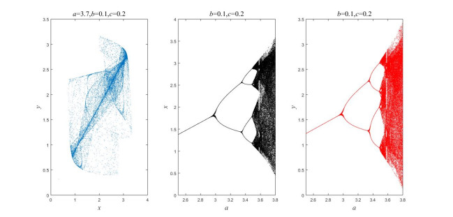
In this paper, the competitive equilibrium of the Bertrand game is discussed with bounded rationality and the utility function. When the parameters changing and the number of firms increasing, the competitive equilibrium valve of Bertrand duopoly game is gradually being blurred. When the number of competitors is more than four, it is very difficult to derive the value of the equilibrium points. How to find the general competitive equilibrium points for Bertrand game, which is studied from spatial agglomeration with mean value theorem. A Bertrand duopoly game is proposed based on a demand function. Celestial bodies motion as method is introduced to handle the number and stability of competitive equilibrium points, and the stable points is symmetry. The results are supported by numerical computation and simulations.

Keywords:

Citation: Bingyuan Gao, Yaxin Zheng, Jieyu Huang. General equilibrium of Bertrand game: A spatial computational approach[J]. AIMS Mathematics, 2021, 6(9): 10025-10036. doi: 10.3934/math.2021582

Related Papers:

[1]	Ahmed Ghezal, Mohamed Balegh, Imane Zemmouri . Solutions and local stability of the Jacobsthal system of difference equations. AIMS Mathematics, 2024, 9(2): 3576-3591. doi: 10.3934/math.2024175
[2]	Hashem Althagafi, Ahmed Ghezal . Solving a system of nonlinear difference equations with bilinear dynamics. AIMS Mathematics, 2024, 9(12): 34067-34089. doi: 10.3934/math.20241624
[3]	M. T. Alharthi . Correction: On the solutions of some systems of rational difference equations. AIMS Mathematics, 2025, 10(2): 2277-2278. doi: 10.3934/math.2025105
[4]	M. T. Alharthi . On the solutions of some systems of rational difference equations. AIMS Mathematics, 2024, 9(11): 30320-30347. doi: 10.3934/math.20241463
[5]	Eunjung Lee, Dojin Kim . Stability analysis of the implicit finite difference schemes for nonlinear Schrödinger equation. AIMS Mathematics, 2022, 7(9): 16349-16365. doi: 10.3934/math.2022893
[6]	Shulan Kong, Chengbin Wang, Yawen Sun . A recursive filter for a class of two-dimensional nonlinear stochastic systems. AIMS Mathematics, 2025, 10(1): 1741-1756. doi: 10.3934/math.2025079
[7]	Yeyang Jiang, Zhihua Liao, Di Qiu . The existence of entire solutions of some systems of the Fermat type differential-difference equations. AIMS Mathematics, 2022, 7(10): 17685-17698. doi: 10.3934/math.2022974
[8]	Abdulghani R. Alharbi . Traveling-wave and numerical solutions to nonlinear evolution equations via modern computational techniques. AIMS Mathematics, 2024, 9(1): 1323-1345. doi: 10.3934/math.2024065
[9]	Ibraheem M. Alsulami, E. M. Elsayed . On a class of nonlinear rational systems of difference equations. AIMS Mathematics, 2023, 8(7): 15466-15485. doi: 10.3934/math.2023789
[10]	Nan Li, Jiachuan Geng, Lianzhong Yang . Some results on transcendental entire solutions to certain nonlinear differential-difference equations. AIMS Mathematics, 2021, 6(8): 8107-8126. doi: 10.3934/math.2021470

Abstract

1. Introduction

This paper is devoted to study the expressions forms of the solutions and periodic nature of the following third-order rational systems of difference equations

$\begin{equation*} x_{n+1} = \dfrac{y_{n-1}z_{n}}{z_{n}\pm x_{n-2}}, \;y_{n+1} = \dfrac{z_{n-1}x_{n} }{x_{n}\pm y_{n-2}}, \ z_{n+1} = \dfrac{x_{n-1}y_{n}}{y_{n}\pm z_{n-2}}, \end{equation*}$

with initial conditions are non-zero real numbers.

In the recent years, there has been great concern in studying the systems of difference equations. One of the most important reasons for this is a exigency for some mechanization which can be used in discussing equations emerge in mathematical models characterizing real life situations in economic, genetics, probability theory, psychology, population biology and so on.

Difference equations display naturally as discrete peer and as numerical solutions of differential equations having more applications in ecology, biology, physics, economy, and so forth. For all that the difference equations are quite simple in expressions, it is frequently difficult to realize completely the dynamics of their solutions see ^{[1,2,3,4,5,6,7,8,9,10,11,12,13,14,15,16,17,18,19]} and the related references therein.

There are some papers dealed with the difference equations systems, for example, The periodic nature of the solutions of the nonlinear difference equations system

$\begin{equation*} A_{n+1} = \dfrac{1}{C_{n}}, \;B_{n+1} = \dfrac{B_{n}}{A_{n-1}B_{n-1}}, \;C_{n+1} = \dfrac{1}{A_{n-1}}, \end{equation*}$

has been studied by Cinar in ^[7].

Almatrafi ^[3] determined the analytical solutions of the following systems of rational recursive equations

$\begin{equation*} x_{n+1} = \dfrac{x_{n-1}y_{n-3}}{y_{n-1}(\pm 1\pm x_{n-1}y_{n-3})}, \;y_{n+1} = \dfrac{y_{n-1}x_{n-3}}{x_{n-1}(\pm 1\pm y_{n-1}x_{n-3})}. \end{equation*}$

In ^[20], Khaliq and Shoaib studied the local and global asymptotic behavior of non-negative equilibrium points of a three-dimensional system of two order rational difference equations

$\begin{equation*} x_{n+1} = \dfrac{x_{n-1}}{\varepsilon +x_{n-1}y_{n-1}z_{n-1}}, \;y_{n+1} = \dfrac{ y_{n-1}}{\zeta +x_{n-1}y_{n-1}z_{n-1}}, \ z_{n+1} = \dfrac{z_{n-1}}{\eta +x_{n-1}y_{n-1}z_{n-1}}. \end{equation*}$

In ^[9], Elabbasy et al. obtained the form of the solutions of some cases of the following system of difference equations

$\begin{eqnarray*} x_{n+1} & = &\dfrac{a_{1}+a_{2}y_{n}}{a_{3}z_{n}+a_{4}x_{n-1}z_{n}}, \ y_{n+1} = \dfrac{b_{1}z_{n-1}+b_{2}z_{n}}{b_{3}x_{n}y_{n}+b_{4}x_{n}y_{n-1}}, \\ z_{n+1} & = &\dfrac{c_{1}z_{n-1}+c_{2}z_{n}}{ c_{3}x_{n-1}y_{n-1}+c_{4}x_{n-1}y_{n}+c_{5}x_{n}y_{n}}. \end{eqnarray*}$

In ^[12], Elsayed et al. have got the solutions of the systems of rational higher order difference equations

$\begin{equation*} A_{n+1} = \dfrac{1}{A_{n-p}B_{n-p}}, \;\;B_{n+1} = \dfrac{A_{n-p}B_{n-p}}{ A_{n-q}B_{n-q}}, \end{equation*}$

and

$\begin{equation*} A_{n+1} = \dfrac{1}{A_{n-p}B_{n-p}C_{n-p}}, \;\;B_{n+1} = \dfrac{ A_{n-p}B_{n-p}C_{n-p}}{A_{n-q}B_{n-q}C_{n-q}}, \;C_{n+1} = \dfrac{ A_{n-q}B_{n-q}C_{n-q}}{A_{n-r}B_{n-r}C_{n-r}}. \end{equation*}$

Kurbanli ^[25,26] investigated the behavior of the solutions of the following systems

$\begin{eqnarray*} A_{n+1} & = &\dfrac{A_{n-1}}{A_{n-1}B_{n}-1}, \;B_{n+1} = \dfrac{B_{n-1}}{ B_{n-1}A_{n}-1}, \ \ C_{n+1} = \dfrac{1}{C_{n}B_{n}}, \\ A_{n+1} & = &\dfrac{A_{n-1}}{A_{n-1}B_{n}-1}, \;B_{n+1} = \dfrac{B_{n-1}}{ B_{n-1}A_{n}-1}, \ \ C_{n+1} = \dfrac{C_{n-1}}{C_{n-1}B_{n}-1}. \end{eqnarray*}$

In ^[32], Yalçınkaya has obtained the conditions for the global asymptotically stable of the system

$\begin{equation*} A_{n+1} = \dfrac{B_{n}A_{n-1}+a}{B_{n}+A_{n-1}}, \;B_{n+1} = \dfrac{A_{n}B_{n-1}+a }{A_{n}+B_{n-1}}. \end{equation*}$

Zhang et al. ^[39] investigated the persistence, boundedness and the global asymptotically stable of the solutions of the following system

$\begin{equation*} R_{n} = A+\dfrac{1}{Q_{n-p}}, \ \ \ \;Q_{n} = A+\dfrac{Q_{n-1}}{R_{n-r}Q_{n-s}}. \end{equation*}$

Similar to difference equations and systems were studied see ^{[21,22,23,24,27,28,29,30,31,32,33,34,35,36,37,38]}.

2. The system: $x_{n+1}=\dfrac{y_{n-1}z_{n}}{z_{n}+x_{n-2}}, \; y_{n+1}= \dfrac{z_{n-1}x_{n}}{x_{n}+y_{n-2}},$ $z_{n+1}=\dfrac{x_{n-1}y_{n}}{ y_{n}+z_{n-2}}$

In this section, we obtain the expressions form of the solutions of the following three dimension system of difference equations

$\begin{equation} x_{n+1} = \dfrac{y_{n-1}z_{n}}{z_{n}+x_{n-2}}, \;y_{n+1} = \dfrac{z_{n-1}x_{n}}{ x_{n}+y_{n-2}}, \ z_{n+1} = \dfrac{x_{n-1}y_{n}}{y_{n}+z_{n-2}}, \end{equation}$

(1)

where $n\in \mathbb{N}_{0}$ and the initial conditions are non-zero real numbers.

Theorem 1. We assume that $\{x_{n}, y_{n}, z_{n}\}$ are solutions of system (1).Then

$\begin{eqnarray*} x_{6n-2} & = &\frac{ak^{3n}}{\prod \limits_{i = 0}^{n-1}(a+(6i)k)(a+(6i+2)k)(a+(6i+4)k)}, \\ x_{6n-1} & = &\frac{bf^{3n}}{\prod \limits_{i = 0}^{n-1}(g+(6i+1)f)(g+(6i+3)f)(g+(6i+5)f)}, \\ x_{6n} & = &\frac{c^{3n+1}}{\prod \limits_{i = 0}^{n-1}(d+(6i+2)c)(d+(6i+4)c)(d+(6i+6)c)}, \\ x_{6n+1} & = &\frac{ek^{3n+1}}{(a+k)\prod \limits_{i = 0}^{n-1}(a+(6i+3)k)(a+(6i+5)k)(a+(6i+7)k)}, \end{eqnarray*}$

$\begin{eqnarray*} x_{6n+2} & = &\frac{f^{3n+2}}{(g+2f)\prod \limits_{i = 0}^{n-1}(g+(6i+4)f)(g+(6i+6)f)(g+(6i+8)f)}, \\ x_{6n+3} & = &\frac{hc^{3n+2}}{(d+c)(d+3c)\prod \limits_{i = 0}^{n-1}(d+(6i+5)c)(d+(6i+7)c)(d+(6i+9)c)}, \end{eqnarray*}$

$\begin{eqnarray*} y_{6n-2} & = &\frac{dc^{3n}}{\prod \limits_{i = 0}^{n-1}(d+(6i)c)(d+(6i+2)c)(d+(6i+4)c)}, \\ y_{6n-1} & = &\frac{ek^{3n}}{\prod \limits_{i = 0}^{n-1}(a+(6i+1)k)(a+(6i+3)k)(a+(6i+5)k)}, \\ y_{6n} & = &\frac{f^{3n+1}}{\prod \limits_{i = 0}^{n-1}(g+(6i+2)f)(g+(6i+4)f)(g+(6i+6)f)}, \\ y_{6n+1} & = &\frac{hc^{3n+1}}{(d+c)\prod \limits_{i = 0}^{n-1}(d+(6i+3)c)(d+(6i+5)c)(d+(6i+7)c)}, \\ y_{6n+2} & = &\frac{k^{3n+2}}{(a+2k)\prod \limits_{i = 0}^{n-1}(a+(6i+4)k)(a+(6i+6)k)(a+(6i+8)k)}, \\ y_{6n+3} & = &\frac{bf^{3n+2}}{(g+f)(g+3f)\prod \limits_{i = 0}^{n-1}(g+(6i+5)f)(g+(6i+7)f)(g+(6i+9)f)}, \end{eqnarray*}$

and

$\begin{eqnarray*} z_{6n-2} & = &\frac{gf^{3n}}{\prod \limits_{i = 0}^{n-1}(g+(6i)f)(g+(6i+2)f)(g+(6i+4)f)}, \\ z_{6n-1} & = &\frac{hc^{3n}}{\prod \limits_{i = 0}^{n-1}(d+(6i+1)c)(d+(6i+3)c)(d+(6i+5)c)}, \\ z_{6n} & = &\frac{k^{3n+1}}{\prod \limits_{i = 0}^{n-1}(a+(6i+2)k)(a+(6i+4)k)(a+(6i+6)k)}, \\ z_{6n+1} & = &\frac{bf^{3n+1}}{(g+f)\prod \limits_{i = 0}^{n-1}(g+(6i+3)f)(g+(6i+5)f)(g+(6i+7)f)}, \end{eqnarray*}$

$\begin{eqnarray*} z_{6n+2} & = &\frac{c^{3n+2}}{(d+2c)\prod \limits_{i = 0}^{n-1}(d+(6i+4)c)(d+(6i+6)c)(d+(6i+8)c)}, \\ z_{6n+3} & = &\frac{ek^{3n+2}}{(a+k)(a+3k)\prod \limits_{i = 0}^{n-1}(a+(6i+5)k)(a+(6i+7)k)(a+(6i+9)k)}, \end{eqnarray*}$

where $x_{-2} = a, \ x_{-1} = b,$ $x_{0} = c,$ $y_{-2} = d,$ $y_{-1} = e,$ $y_{0} = f,$ $z_{-2} = g,$ $z_{-1} = h$ $and$ $z_{0} = k.$

Proof. For $n = 0$ the result holds. Now assume that $n > 1$ and that our assumption holds for $n-1$ , that is,

$\begin{eqnarray*} x_{6n-8} & = &\frac{ak^{3n-3}}{\prod \limits_{i = 0}^{n-2}(a+(6i)k)(a+(6i+2)k)(a+(6i+4)k)}, \\ x_{6n-7} & = &\frac{bf^{3n-3}}{\prod \limits_{i = 0}^{n-2}(g+(6i+1)f)(g+(6i+3)f)(g+(6i+5)f)}, \\ x_{6n-6} & = &\frac{c^{3n-2}}{\prod \limits_{i = 0}^{n-2}(d+(6i+2)c)(d+(6i+4)c)(d+(6i+6)c)}, \\ x_{6n-5} & = &\frac{ek^{3n-2}}{(a+k)\prod \limits_{i = 0}^{n-2}(a+(6i+3)k)(a+(6i+5)k)(a+(6i+7)k)}, \\ x_{6n-4} & = &\frac{f^{3n-1}}{(g+2f)\prod \limits_{i = 0}^{n-2}(g+(6i+4)f)(g+(6i+6)f)(g+(6i+8)f)}, \\ x_{6n-3} & = &\frac{hc^{3n-1}}{(d+c)(d+3c)\prod \limits_{i = 0}^{n-2}(d+(6i+5)c)(d+(6i+7)c)(d+(6i+9)c)}, \end{eqnarray*}$

$\begin{eqnarray*} y_{6n-8} & = &\frac{dc^{3n-3}}{\prod \limits_{i = 0}^{n-2}(d+(6i)c)(d+(6i+2)c)(d+(6i+4)c)}, \\ y_{6n-7} & = &\frac{ek^{3n-3}}{\prod \limits_{i = 0}^{n-2}(a+(6i+1)k)(a+(6i+3)k)(a+(6i+5)k)}, \\ y_{6n-6} & = &\frac{f^{3n-2}}{\prod \limits_{i = 0}^{n-2}(g+(6i+2)f)(g+(6i+4)f)(g+(6i+6)f)}, \end{eqnarray*}$

$\begin{eqnarray*} y_{6n-5} & = &\frac{hc^{3n-2}}{(d+c)\prod \limits_{i = 0}^{n-2}(d+(6i+3)c)(d+(6i+5)c)(d+(6i+7)c)}, \\ y_{6n-4} & = &\frac{k^{3n-1}}{(a+2k)\prod \limits_{i = 0}^{n-2}(a+(6i+4)k)(a+(6i+6)k)(a+(6i+8)k)}, \\ y_{6n-3} & = &\frac{bf^{3n-1}}{(g+f)(g+3f)\prod \limits_{i = 0}^{n-2}(g+(6i+5)f)(g+(6i+7)f)(g+(6i+9)f)}, \end{eqnarray*}$

and

$\begin{eqnarray*} z_{6n-8} & = &\frac{gf^{3n-3}}{\prod \limits_{i = 0}^{n-2}(g+(6i)f)(g+(6i+2)f)(g+(6i+4)f)}, \\ z_{6n-7} & = &\frac{hc^{3n-3}}{\prod \limits_{i = 0}^{n-2}(d+(6i+1)c)(d+(6i+3)c)(d+(6i+5)c)}, \\ z_{6n-6} & = &\frac{k^{3n-2}}{\prod \limits_{i = 0}^{n-2}(a+(6i+2)k)(a+(6i+4)k)(a+(6i+6)k)}, \\ z_{6n-5} & = &\frac{bf^{3n-2}}{(g+f)\prod \limits_{i = 0}^{n-2}(g+(6i+3)f)(g+(6i+5)f)(g+(6i+7)f)}, \\ z_{6n-4} & = &\frac{c^{3n-1}}{(d+2c)\prod \limits_{i = 0}^{n-2}(d+(6i+4)c)(d+(6i+6)c)(d+(6i+8)c)}, \\ z_{6n-3} & = &\frac{ek^{3n-1}}{(a+k)(a+3k)\prod \limits_{i = 0}^{n-2}(a+(6i+5)k)(a+(6i+7)k)(a+(6i+9)k)}. \end{eqnarray*}$

It follows from Eq (1) that

$\begin{eqnarray*} x_{6n-2} & = &\dfrac{y_{6n-4}z_{6n-3}}{z_{6n-3}+x_{6n-5}} \\ & = &\tfrac{\left( \frac{k^{3n-1}}{(a+2k)\prod \limits_{i = 0}^{n-2}(a+(6i+4)k)(a+(6i+6)k)(a+(6i+8)k)}\ \ \ \ \ \ \ \ \ \ \ \ \ \ \ \ \ \ \ \ \ \ \ \ \ \ \ \ \right) \left( \frac{ ek^{3n-1}}{(a+k)(a+3k)\prod \limits_{i = 0}^{n-2}(a+(6i+5)k)(a+(6i+7)k)(a+(6i+9)k)}\ \ \ \ \ \ \ \ \ \ \ \ \ \ \ \ \ \ \ \ \ \ \ \ \ \ \ \ \right) }{\left( \frac{ ek^{3n-1}}{(a+k)(a+3k)\prod \limits_{i = 0}^{n-2}(a+(6i+5)k)(a+(6i+7)k)(a+(6i+9)k)}\ \ \ \ \ \ \ \ \ \ \ \ \ \ \ \ \ \ \ \ \ \ \ \ \ \ \ \ \right) +\left( \frac{ ek^{3n-2}}{(a+k)\prod\limits_{i = 0}^{n-2}(a+(6i+3)k)(a+(6i+5)k)(a+(6i+7)k)}\ \ \ \ \ \ \ \ \ \ \ \ \ \ \ \ \ \ \ \ \ \ \ \ \ \ \ \ \right) } \\ & = &\dfrac{\left( \frac{k^{3n}}{(a+2k)\prod \limits_{i = 0}^{n-2}(a+(6i+4)k)(a+(6i+6)k)(a+(6i+8)k)}\right) }{ (a+3k)\prod\limits_{i = 0}^{n-2}(a+(6i+9)k)\left[ \left( \frac{k}{ (a+3k)\prod\limits_{i = 0}^{n-2}(a+(6i+9)k)}\right) +\left( \frac{1}{ \prod\limits_{i = 0}^{n-2}(a+(6i+3)k)}\right) \right] } \\ & = &\dfrac{\left( \frac{k^{3n}}{(a+2k)\prod \limits_{i = 0}^{n-2}(a+(6i+4)k)(a+(6i+6)k)(a+(6i+8)k)}\right) }{\left[ k+\left( \frac{(a+3k)\prod\limits_{i = 0}^{n-2}(a+(6i+9)k)}{ \prod\limits_{i = 0}^{n-2}(a+(6i+3)k)}\right) \right] } \\ & = &\dfrac{\left( \frac{k^{3n}}{(a+2k)\prod \limits_{i = 0}^{n-2}(a+(6i+4)k)(a+(6i+6)k)(a+(6i+8)k)}\right) }{\left[ k+\left( a+(6n-3)k\right) \right] } \\ & = &\frac{ak^{3n}}{a(a+2k)\left( a+(6n-2)k\right) \prod\limits_{i = 0}^{n-2}(a+(6i+4)k)(a+(6i+6)k)(a+(6i+8)k)}. \end{eqnarray*}$

Then we see that

$\begin{equation*} x_{6n-2} = \frac{k^{3n}}{\prod \limits_{i = 0}^{n-1}(a+(6i)k)(a+(6i+2)k)(a+(6i+4)k)}. \end{equation*}$

Also, we see from Eq (1) that

$\begin{eqnarray*} y_{6n-2} & = &\dfrac{z_{6n-4}x_{6n-3}}{x_{6n-3}+y_{6n-5}} \\ & = &\tfrac{\left( \frac{c^{3n-1}}{(d+2c)\prod \limits_{i = 0}^{n-2}(d+(6i+4)c)(d+(6i+6)c)(d+(6i+8)c)}\ \ \ \ \ \ \ \ \ \ \ \ \ \ \ \ \ \ \ \ \ \ \ \ \ \right) \left( \frac{ hc^{3n-1}}{(d+c)(d+3c)\prod \limits_{i = 0}^{n-2}(d+(6i+5)c)(d+(6i+7)c)(d+(6i+9)c)}\ \ \ \ \ \ \ \ \ \ \ \ \ \ \ \ \ \ \ \ \ \ \ \ \ \right) }{\left( \frac{ hc^{3n-1}}{(d+c)(d+3c)\prod \limits_{i = 0}^{n-2}(d+(6i+5)c)(d+(6i+7)c)(d+(6i+9)c)}\ \ \ \ \ \ \ \ \ \ \ \ \ \ \ \ \ \ \ \ \ \ \ \ \ \right) +\left( \frac{ hc^{3n-2}}{(d+c)\prod\limits_{i = 0}^{n-2}(d+(6i+3)c)(d+(6i+5)c)(d+(6i+7)c)} \ \ \ \ \ \ \ \ \ \ \ \ \ \ \ \ \ \ \ \ \ \ \ \ \ \right) } \\ & = &\dfrac{\left( \frac{c^{3n}}{(d+2c)\prod \limits_{i = 0}^{n-2}(d+(6i+4)c)(d+(6i+6)c)(d+(6i+8)c)}\right) }{ (d+3c)\prod\limits_{i = 0}^{n-2}(d+(6i+9)c)\left[ \left( \frac{c}{ (d+3c)\prod\limits_{i = 0}^{n-2}(d+(6i+9)c)}\right) +\left( \frac{1}{ \prod\limits_{i = 0}^{n-2}(d+(6i+3)c)}\right) \right] } \\ & = &\dfrac{\left( \frac{c^{3n}}{(d+2c)\prod \limits_{i = 0}^{n-2}(d+(6i+4)c)(d+(6i+6)c)(d+(6i+8)c)}\right) }{\left[ c+d+(6n-3)c\right] } \\ & = &\dfrac{c^{3n}}{\left[ d+(6n-2)c\right] (d+2c)\prod \limits_{i = 0}^{n-2}(d+(6i+4)c)(d+(6i+6)c)(d+(6i+8)c)}. \end{eqnarray*}$

Then

$\begin{equation*} y_{6n-2} = \dfrac{dc^{3n}}{\prod \limits_{i = 0}^{n-1}(d+(6i)c)(d+(6i+2)c)(d+(6i+4)c)}. \end{equation*}$

Finally from Eq (1), we see that

$\begin{eqnarray*} z_{6n-2} & = &\dfrac{x_{6n-4}y_{6n-3}}{y_{6n-3}+z_{6n-5}} \\ & = &\tfrac{\left( \frac{f^{3n-1}}{(g+2f)\prod \limits_{i = 0}^{n-2}(g+(6i+4)f)(g+(6i+6)f)(g+(6i+8)f)}\ \ \ \ \ \ \ \ \ \ \ \ \ \ \ \ \ \ \ \ \ \ \ \ \ \ \ \ \right) \left( \frac{ bf^{3n-1}}{(g+f)(g+3f)\prod \limits_{i = 0}^{n-2}(g+(6i+5)f)(g+(6i+7)f)(g+(6i+9)f)}\ \ \ \ \ \ \ \ \ \ \ \ \ \ \ \ \ \ \ \ \ \ \ \ \ \ \ \ \right) }{\left( \frac{ bf^{3n-1}}{(g+f)(g+3f)\prod \limits_{i = 0}^{n-2}(g+(6i+5)f)(g+(6i+7)f)(g+(6i+9)f)}\ \ \ \ \ \ \ \ \ \ \ \ \ \ \ \ \ \ \ \ \ \ \ \ \ \ \ \ \right) +\left( \frac{ bf^{3n-2}}{(g+f)\prod\limits_{i = 0}^{n-2}(g+(6i+3)f)(g+(6i+5)f)(g+(6i+7)f)} \ \ \ \ \ \ \ \ \ \ \ \ \ \ \ \ \ \ \ \ \ \ \ \ \ \ \ \ \right) } \\ & = &\dfrac{\left( \frac{f^{3n}}{(g+2f)\prod \limits_{i = 0}^{n-2}(g+(6i+4)f)(g+(6i+6)f)(g+(6i+8)f)}\right) }{ (g+3f)\prod\limits_{i = 0}^{n-2}(g+(6i+9)f)\left[ \left( \frac{f}{ (g+3f)\prod\limits_{i = 0}^{n-2}(g+(6i+9)f)}\right) +\left( \frac{1}{ \prod\limits_{i = 0}^{n-2}(g+(6i+3)f)}\right) \right] } \\ & = &\dfrac{\left( \frac{f^{3n}}{(g+2f)\prod \limits_{i = 0}^{n-2}(g+(6i+4)f)(g+(6i+6)f)(g+(6i+8)f)}\right) }{\left[ f+\left( \frac{(g+3f)\prod\limits_{i = 0}^{n-2}(g+(6i+9)f)}{ \prod\limits_{i = 0}^{n-2}(g+(6i+3)f)}\right) \right] } \\ & = &\dfrac{\left( \frac{f^{3n}}{(g+2f)\prod \limits_{i = 0}^{n-2}(g+(6i+4)f)(g+(6i+6)f)(g+(6i+8)f)}\right) }{\left[ f+(g+(6n-3)f)\right] } \\ & = &\dfrac{f^{3n}}{(g+(6n-2)f)(g+2f)\prod \limits_{i = 0}^{n-2}(g+(6i+4)f)(g+(6i+6)f)(g+(6i+8)f)}. \end{eqnarray*}$

Thus

$\begin{equation*} z_{3n-2} = \dfrac{gf^{3n}}{\prod \limits_{i = 0}^{n-1}(g+(6i)f)(g+(6i+2)f)(g+(6i+4)f)}. \end{equation*}$

By similar way, one can show the other relations. This completes the proof.

Lemma 1. Let $\{x_{n}, y_{n}, z_{n}\}$ be a positive solution of system (1), then all solution of (1) is bounded and approaching to zero.

Proof. It follows from Eq (1) that

$\begin{eqnarray*} x_{n+1} & = &\dfrac{y_{n-1}z_{n}}{z_{n}+x_{n-2}}\leq y_{n-1}, \ \ \ \ \ y_{n+1} = \dfrac{z_{n-1}x_{n}}{x_{n}+y_{n-2}}\leq z_{n-1}, \\ z_{n+1} & = &\dfrac{x_{n-1}y_{n}}{y_{n}+z_{n-2}}\leq x_{n-1}, \end{eqnarray*}$

we see that

$\begin{eqnarray*} x_{n+4} &\leq &y_{n+2}, \ \ \ \ \ y_{n+2}\leq z_{n}, \ \ z_{n}\leq x_{n-2}, \ \ \ \Rightarrow \ x_{n+4} < x_{n-2}, \\ y_{n+4} &\leq &z_{n+2}, \ \ \ z_{n+2}\leq x_{n}, \ \ \ x_{n}\leq y_{n-2}, \ \ \ \ \ \Rightarrow \ y_{n+4} < y_{n-2}, \\ z_{n+4} &\leq &x_{n+2}, \ \ \ x_{n+2}\leq y_{n}, \ \ \ y_{n}\leq z_{n-2}, \ \ \ \ \ \Rightarrow \ z_{n+4} < z_{n-2}, \end{eqnarray*}$

Then all subsequences of $\{x_{n}, y_{n}, z_{n}\}$ (i.e., for $\{x_{n}\}$ are $\{x_{6n-2}\}$ , $\{x_{6n-1}\}$ , $\{x_{6n}\},$ $\{x_{6n+1}\}$ , $\{x_{6n+2}\}$ , $\{x_{6n+3}\}\$ are decreasing and at that time are bounded from above by $K, L$ and $M$ since $K = \max \{x_{-2}, x_{-1}, x_{0}, x_{1}, x_{2}, x_{3}\},$ $L = \max \{y_{-2}, y_{-1}, y_{0}, y_{1}, y_{2}, y_{3}\}$ and $M = \max \{z_{-2}, z_{-1}, z_{0}, z_{1}, z_{2}, z_{3}\}$ .

Example 1. We assume an interesting numerical example for the system (1) with $x_{-2} = -.22, \; x_{-1} = -.4, \ x_{0} = .12, \; y_{-2} = -.62,$ $y_{-1} = 4, \ y_{0} = .3, \; z_{-2} = .4, \; z_{-1} = .53\ and\; z_{0} = -2$ . (See Figure 1).

Figure 1. This figure shows the behavior of the solutions of the system (1) with the initial conditions

$x_{-2} = -.22, \; x_{-1} = -.4, \ x_{0} = .12, \; y_{-2} = -.62,$

$y_{-1} = 4, \ y_{0} = .3, \; z_{-2} = .4, \; z_{-1} = .53\ and\; z_{0} = -2.$ (We see from this figure that all solutions converges to zero).

DownLoad: Full-Size Img PowerPoint

3. The system: $x_{n+1}=\dfrac{y_{n-1}z_{n}}{z_{n}+x_{n-2}}, \; y_{n+1}= \dfrac{z_{n-1}x_{n}}{x_{n}+y_{n-2}},$ $z_{n+1}=\dfrac{x_{n-1}y_{n}}{ y_{n}-z_{n-2}}$

In this section, we get the solution's form of the following system of difference equations

$\begin{equation} x_{n+1} = \dfrac{y_{n-1}z_{n}}{z_{n}+x_{n-2}}, \;y_{n+1} = \dfrac{z_{n-1}x_{n}}{ x_{n}+y_{n-2}}, \ z_{n+1} = \dfrac{x_{n-1}y_{n}}{y_{n}-z_{n-2}}, \end{equation}$

(2)

where $n\in \mathbb{N}_{0}$ and the initial values are non-zero real numbers with $x_{-2}\neq \pm z_{0}, \neq -2z_{0},$ $z_{-2}\neq y_{0}, \neq 2y_{0}, \neq 3y_{0}$ and $y_{-2}\neq 2x_{0}, \neq \pm x_{0}.$

Theorem 2. Assume that $\{x_{n}, y_{n}, z_{n}\}$ are solutions of (2). Then for $n = 0, 1, 2, ...,$

$\begin{eqnarray*} x_{6n-2} & = &\frac{(-1)^{n}k^{3n}}{a^{2n-1}(a+2k)^{n}}, \ x_{6n-1} = \frac{ (-1)^{n}bf^{3n}}{(f-g)^{2n}(3f-g)^{n}}, \ x_{6n} = \frac{(-1)^{n}c^{3n+1}}{ d^{2n}(2c-d)^{n}}, \\ x_{6n+1} & = &\frac{ek^{3n+1}}{(a-k)^{n}(a+k)^{2n+1}}, \ x_{6n+2} = \frac{ (-1)^{n}f^{3n+2}}{g^{n}(2f-g)^{2n+1}}, \ x_{6n+3} = \frac{(-1)^{n}hc^{3n+2}}{ (c-d)^{2n+1}(c+d)^{n+1}}, \end{eqnarray*}$

$\begin{eqnarray*} y_{6n-2} & = &\frac{(-1)^{n}c^{3n}}{d^{2n-1}(2c-d)^{n}}, \ y_{6n-1} = \frac{ ek^{3n}}{(a-k)^{n}(a+k)^{2n}}, \ y_{6n} = \frac{(-1)^{n}f^{3n+1}}{ g^{n}(2f-g)^{2n}}, \\ y_{6n+1} & = &\frac{(-1)^{n}hc^{3n+1}}{(c-d)^{2n}(c+d)^{n+1}}, \ y_{6n+2} = \frac{ (-1)^{n}k^{3n+2}}{a^{2n}(a+2k)^{n+1}}, \ y_{6n+3} = \frac{(-1)^{n}bf^{3n+2}}{ (f-g)^{2n+1}(3f-g)^{n+1}}, \end{eqnarray*}$

and

$\begin{eqnarray*} z_{6n-2} & = &\frac{(-1)^{n}f^{3n}}{g^{n-1}(2f-g)^{2n}}, \ z_{6n-1} = \frac{ (-1)^{n}hc^{3n}}{(c-d)^{2n}(c+d)^{n}}, \ z_{6n} = \frac{(-1)^{n}k^{3n+1}}{ a^{2n}(a+2k)^{n}}, \\ z_{6n+1} & = &\frac{(-1)^{n}bf^{3n+1}}{(f-g)^{2n+1}(3f-g)^{n}}, \ z_{6n+2} = \frac{(-1)^{n+1}c^{3n+2}}{d^{2n+1}(2c-d)^{n}}, \ z_{6n+3} = \frac{-ek^{3n+2}}{ (a-k)^{n}(a+k)^{2n+2}}, \end{eqnarray*}$

where $x_{-2} = a, \ x_{-1} = b,$ $x_{0} = c,$ $y_{-2} = d,$ $y_{-1} = e,$ $y_{0} = f,$ $z_{-2} = g,$ $z_{-1} = h$ $and$ $z_{0} = k.$

Proof. The result is true for $n = 0$ . Now suppose that $n > 0$ and that our claim verified for $n-1$ . That is,

$\begin{eqnarray*} x_{6n-8} & = &\frac{(-1)^{n-1}k^{3n-3}}{a^{2n-3}(a+2k)^{n-1}}, \ x_{6n-7} = \frac{ (-1)^{n-1}bf^{3n-3}}{(f-g)^{2n-2}(3f-g)^{n-1}}, \ x_{6n-6} = \frac{ (-1)^{n-1}c^{3n-2}}{d^{2n-2}(2c-d)^{n-1}}, \\ x_{6n-5} & = &\frac{ek^{3n-2}}{(a-k)^{n-1}(a+k)^{2n-1}}, \ x_{6n-4} = \frac{ (-1)^{n-1}f^{3n-1}}{g^{n-1}(2f-g)^{2n-1}}, \ x_{6n-3} = \frac{ (-1)^{n-1}hc^{3n-1}}{(c-d)^{2n-1}(c+d)^{n}}, \end{eqnarray*}$

$\begin{eqnarray*} y_{6n-8} & = &\frac{(-1)^{n-1}c^{3n-3}}{d^{2n-3}(2c-d)^{n-1}}, \ y_{6n-7} = \frac{ ek^{3n-3}}{(a-k)^{n-1}(a+k)^{2n-2}}, \ y_{6n-6} = \frac{(-1)^{n-1}f^{3n-2}}{ g^{n-1}(2f-g)^{2n-2}}, \\ y_{6n-5} & = &\frac{(-1)^{n-1}hc^{3n-2}}{(c-d)^{2n-2}(c+d)^{n}}, \ y_{6n-4} = \frac{(-1)^{n-1}k^{3n-1}}{a^{2n-2}(a+2k)^{n}}, \ y_{6n-3} = \frac{ (-1)^{n-1}bf^{3n-1}}{(f-g)^{2n-1}(3f-g)^{n}}, \end{eqnarray*}$

and

$\begin{eqnarray*} z_{6n-8} & = &\frac{(-1)^{n-1}f^{3n-3}}{g^{n-2}(2f-g)^{2n-2}}, \ z_{6n-7} = \frac{ (-1)^{n-1}hc^{3n-3}}{(c-d)^{2n-2}(c+d)^{n-1}}, \ z_{6n-6} = \frac{ (-1)^{n-1}k^{3n-2}}{a^{2n-2}(a+2k)^{n-1}}, \\ z_{6n-5} & = &\frac{(-1)^{n-1}bf^{3n-2}}{(f-g)^{2n-1}(3f-g)^{n-1}}, \ z_{6n-4} = \frac{(-1)^{n}c^{3n-1}}{d^{2n-1}(2c-d)^{n-1}}, \ z_{6n-3} = \frac{-ek^{3n-1}}{ (a-k)^{n-1}(a+k)^{2n}}. \end{eqnarray*}$

Now from Eq (2), it follows that

$\begin{eqnarray*} x_{6n-2} & = &\dfrac{y_{6n-4}z_{6n-3}}{z_{6n-3}+x_{6n-5}} \\ & = &\dfrac{\left( \dfrac{(-1)^{n-1}k^{3n-1}}{a^{2n-2}(a+2k)^{n}}\right) \left( \dfrac{-ek^{3n-1}}{(a-k)^{n-1}(a+k)^{2n}}\right) }{\left( \dfrac{ -ek^{3n-1}}{(a-k)^{n-1}(a+k)^{2n}}\right) +\left( \dfrac{ek^{3n-2}}{ (a-k)^{n-1}(a+k)^{2n-1}}\right) } \\ & = &\dfrac{\left( \dfrac{(-1)^{n}k^{3n}}{a^{2n-2}(a+2k)^{n}}\right) }{\left( -k+a+k\right) } = \dfrac{(-1)^{n}k^{3n}}{a^{2n-1}(a+2k)^{n}}, \\ y_{6n-2} & = &\dfrac{z_{6n-4}x_{6n-3}}{x_{6n-3}+y_{6n-5}} = \dfrac{\left( \frac{ (-1)^{n}c^{3n-1}}{d^{2n-1}(2c-d)^{n-1}}\right) \left( \frac{ (-1)^{n-1}hc^{3n-1}}{(c-d)^{2n-1}(c+d)^{n}}\right) }{\left( \frac{ (-1)^{n-1}hc^{3n-1}}{(c-d)^{2n-1}(c+d)^{n}}\right) +\left( \frac{ (-1)^{n-1}hc^{3n-2}}{(c-d)^{2n-2}(c+d)^{n}}\right) } \\ & = &\dfrac{\left( \frac{(-1)^{n}c^{3n}}{d^{2n-1}(2c-d)^{n-1}}\right) }{c+c-d} = \frac{(-1)^{n}c^{3n}}{d^{2n-1}(2c-d)^{n}}, \\ z_{6n-2} & = &\dfrac{x_{6n-4}y_{6n-3}}{y_{6n-3}-z_{6n-5}} = \dfrac{\left( \frac{ (-1)^{n-1}f^{3n-1}}{g^{n-1}(2f-g)^{2n-1}}\right) \left( \frac{ (-1)^{n-1}bf^{3n-1}}{(f-g)^{2n-1}(3f-g)^{n}}\right) }{\left( \frac{ (-1)^{n-1}bf^{3n-1}}{(f-g)^{2n-1}(3f-g)^{n}}\right) -\left( \frac{ (-1)^{n-1}bf^{3n-2}}{(f-g)^{2n-1}(3f-g)^{n-1}}\right) } \\ & = &\dfrac{\left( \frac{(-1)^{n-1}f^{3n}}{g^{n-1}(2f-g)^{2n-1}}\right) }{ \left( f-3f+g\right) } = \frac{(-1)^{n}f^{3n}}{g^{n-1}(2f-g)^{2n}}. \end{eqnarray*}$

Also, we see from Eq (2) that

$\begin{eqnarray*} x_{6n-1} & = &\dfrac{y_{6n-3}z_{6n-2}}{z_{6n-2}+x_{6n-4}} \\ & = &\dfrac{\left( \frac{(-1)^{n-1}bf^{3n-1}}{(f-g)^{2n-1}(3f-g)^{n}}\right) \left( \frac{(-1)^{n}f^{3n}}{g^{n-1}(2f-g)^{2n}}\right) }{\left( \frac{ (-1)^{n}f^{3n}}{g^{n-1}(2f-g)^{2n}}\right) +\left( \frac{(-1)^{n-1}f^{3n-1}}{ g^{n-1}(2f-g)^{2n-1}}\right) } \\ & = &\dfrac{\left( \frac{(-1)^{n}bf^{3n}}{(f-g)^{2n-1}(3f-g)^{n}}\right) }{ \left( -f+2f-g\right) } = \frac{(-1)^{n}bf^{3n}}{(f-g)^{2n}(3f-g)^{n}}, \\ y_{6n-1} & = &\dfrac{z_{6n-3}x_{6n-2}}{x_{6n-2}+y_{6n-4}} = \dfrac{\left( \frac{ -ek^{3n-1}}{(a-k)^{n-1}(a+k)^{2n}}\right) \left( \frac{(-1)^{n}k^{3n}}{ a^{2n-1}(a+2k)^{n}}\right) }{\left( \frac{(-1)^{n}k^{3n}}{a^{2n-1}(a+2k)^{n}} \right) +\left( \frac{(-1)^{n-1}k^{3n-1}}{a^{2n-2}(a+2k)^{n}}\right) } \\ & = &\dfrac{\left( \frac{ek^{3n}}{(a-k)^{n-1}(a+k)^{2n}}\right) }{-k+a} = \frac{ ek^{3n}}{(a-k)^{n}(a+k)^{2n}}, \\ z_{6n-1} & = &\dfrac{x_{6n-3}y_{6n-2}}{y_{6n-2}-z_{6n-4}} = \dfrac{\left( \frac{ (-1)^{n-1}hc^{3n-1}}{(c-d)^{2n-1}(c+d)^{n}}\right) \left( \frac{ (-1)^{n}c^{3n}}{d^{2n-1}(2c-d)^{n}}\right) }{\left( \frac{(-1)^{n}c^{3n}}{ d^{2n-1}(2c-d)^{n}}\right) -\left( \frac{(-1)^{n}c^{3n-1}}{ d^{2n-1}(2c-d)^{n-1}}\right) } \\ & = &\dfrac{\left( \frac{(-1)^{n-1}hc^{3n}}{(c-d)^{2n-1}(c+d)^{n}}\right) }{ c-\left( 2c-d\right) } = \frac{(-1)^{n}hc^{3n}}{(c-d)^{2n}(c+d)^{n}}. \end{eqnarray*}$

Also, we can prove the other relations.

Example 2. See below for system (2) with the initial conditions $x_{-2} = 11, \; x_{-1} = 5, \ x_{0} = 13, \; y_{-2} = 6,$ $y_{-1} = 7, \ y_{0} = 3, \; z_{-2} = 14,$ $z_{-1} = 9$ $and\; z_{0} = 2.$

Figure 2. This figure shows the behavior of solutions of the systems of rational recursive sequence

$x_{n+1} = \dfrac{y_{n-1}z_{n}}{z_{n}+x_{n-2}}, \; y_{n+1} = \dfrac{z_{n-1}x_{n}}{x_{n}+y_{n-2}}, \ z_{n+1} = \dfrac{x_{n-1}y_{n} }{y_{n}-z_{n-2}},$ when we take the initial conditions:

$x_{-2} = 11, \; x_{-1} = 5, \ x_{0} = 13, \; y_{-2} = 6,$

$y_{-1} = 7, \ y_{0} = 3, \; z_{-2} = 14,$

$z_{-1} = 9$

$and\; z_{0} = 2.$ (See the figure we can conclude that all the solutions unboundedness solutions).

DownLoad: Full-Size Img PowerPoint

4. The system: $x_{n+1}=\dfrac{y_{n-1}z_{n}}{z_{n}+x_{n-2}}, \; y_{n+1}= \dfrac{z_{n-1}x_{n}}{x_{n}-y_{n-2}},$ $z_{n+1}=\dfrac{x_{n-1}y_{n}}{ y_{n}+z_{n-2}}$

Here, we obtain the form of solutions of the system

$\begin{equation} x_{n+1} = \dfrac{y_{n-1}z_{n}}{z_{n}+x_{n-2}}, \;y_{n+1} = \dfrac{z_{n-1}x_{n}}{ x_{n}-y_{n-2}}, \ z_{n+1} = \dfrac{x_{n-1}y_{n}}{y_{n}+z_{n-2}}, \end{equation}$

(3)

where $n\in \mathbb{N}_{0}$ and the initial values are non-zero real numbers with $x_{-2}\neq \pm z_{0}, \neq 2z_{0},$ $z_{-2}\neq \pm y_{0}, \neq -2y_{0}$ and $y_{-2}\neq x_{0}, \neq 2x_{0}, \neq 3x_{0}.$

Theorem 3. If $\ \{x_{n}, y_{n}, z_{n}\}$ are solutions of system (3) where $x_{-2} = a, \ x_{-1} = b,$ $x_{0} = c,$ $y_{-2} = d,$ $y_{-1} = e,$ $y_{0} = f,$ $z_{-2} = g,$ $z_{-1} = h$ $and$ $z_{0} = k.$ Then for $n = 0, 1, 2, ...,$

$\begin{eqnarray*} x_{6n-2} & = &\frac{k^{3n}}{a^{2n-1}(a-2k)^{n}}, \ x_{6n-1} = \frac{ (-1)^{n}bf^{3n}}{(f-g)^{n}(f+g)^{2n}}, \ x_{6n} = \frac{(-1)^{n}c^{3n+1}}{ d^{n}(d-2c)^{2n}}, \\ x_{6n+1} & = &\frac{(-1)^{n}ek^{3n+1}}{(a-k)^{2n}(a+k)^{n+1}}, \ x_{6n+2} = \frac{ (-1)^{n}f^{3n+2}}{g^{2n}(2f+g)^{n+1}}, \ x_{6n+3} = \frac{(-1)^{n}hc^{3n+2}}{ (c-d)^{2n+1}(3c-d)^{n+1}}, \end{eqnarray*}$

$\begin{eqnarray*} y_{6n-2} & = &\frac{(-1)^{n}c^{3n}}{d^{n-1}(d-2c)^{2n}}, \ y_{6n-1} = \frac{ (-1)^{n}ek^{3n}}{(a-k)^{2n}(a+k)^{n}}, \ y_{6n} = \frac{(-1)^{n}f^{3n+1}}{ g^{2n}(2f+g)^{n}}, \\ y_{6n+1} & = &\frac{(-1)^{n}hc^{3n+1}}{(c-d)^{2n+1}(3c-d)^{n}}, \ y_{6n+2} = \frac{-k^{3n+2}}{a^{2n+1}(a-2k)^{n}}, \ y_{6n+3} = \frac{(-1)^{n}bf^{3n+2}}{ (f-g)^{n}(f+g)^{2n+2}}, \end{eqnarray*}$

and

$\begin{eqnarray*} z_{6n-2} & = &\frac{(-1)^{n}f^{3n}}{g^{2n-1}(2f+g)^{n}}, \ z_{6n-1} = \frac{ (-1)^{n}hc^{3n}}{(c-d)^{2n}(3c-d)^{n}}, \ z_{6n} = \frac{k^{3n+1}}{ a^{2n}(a-2k)^{n}}, \\ z_{6n+1} & = &\frac{(-1)^{n}bf^{3n+1}}{(f-g)^{n}(f+g)^{2n+1}}, \ z_{6n+2} = \frac{ (-1)^{n}c^{3n+2}}{d^{n}(2c-d)^{2n+1}}, \ z_{6n+3} = \frac{(-1)^{n+1}ek^{3n+2}}{ (a-k)^{2n+1}(a+k)^{n+1}}. \end{eqnarray*}$

Proof. As the proof of Theorem 2 and so will be left to the reader.

Example 3. We put the initials $x_{-2} = 8, \; x_{-1} = 15, \ x_{0} = 13, \; y_{-2} = 6, \; y_{-1} = 7,$ $y_{0} = 3, \; z_{-2} = 14, \; z_{-1} = 19$ $and\; z_{0} = 2,$ for the system (3), see Figure 3.

Figure 3. This figure shows the unstable of the solutions of the difference equations system (3) with the initial values

$x_{-2} = 8, \; x_{-1} = 15, \ x_{0} = 13, \; y_{-2} = 6, \; y_{-1} = 7,$

$y_{0} = 3, \; z_{-2} = 14, \; z_{-1} = 19$

$and\; z_{0} = 2$ .

DownLoad: Full-Size Img PowerPoint

The following systems can be treated similarly.

5. The system: $x_{n+1}=\dfrac{y_{n-1}z_{n}}{z_{n}-x_{n-2}}, \; y_{n+1}= \dfrac{z_{n-1}x_{n}}{x_{n}+y_{n-2}},$ $z_{n+1}=\dfrac{x_{n-1}y_{n}}{ y_{n}+z_{n-2}}$

In this section, we deal with the solutions of the following system

$\begin{equation} x_{n+1} = \dfrac{y_{n-1}z_{n}}{z_{n}-x_{n-2}}, \;y_{n+1} = \dfrac{z_{n-1}x_{n}}{ x_{n}+y_{n-2}}, \ z_{n+1} = \dfrac{x_{n-1}y_{n}}{y_{n}+z_{n-2}}, \end{equation}$

(4)

where $n\in \mathbb{N}_{0}$ and the initial values are non-zero real with $x_{-2}\neq z_{0}, \neq 2z_{0}, \neq 3z_{0},$ $z_{-2}\neq \pm y_{0}, \neq 2y_{0}$ and $y_{-2}\neq \pm x_{0}, \neq -2x_{0}.$

Theorem 4. The solutions of system (4) are given by

$\begin{eqnarray*} x_{6n-2} & = &\frac{(-1)^{n}k^{3n}}{a^{n-1}(a-2k)^{2n}}, \ x_{6n-1} = \frac{ (-1)^{n}bf^{3n}}{(f-g)^{2n}(f+g)^{n}}, \ x_{6n} = \frac{(-1)^{n}c^{3n+1}}{ d^{2n}(d+2c)^{n}}, \\ x_{6n+1} & = &\frac{-ek^{3n+1}}{(a-k)^{2n+1}(a-3k)^{n}}, \ x_{6n+2} = \frac{ (-1)^{n+1}f^{3n+2}}{g^{2n+1}(2f-g)^{n}}, \ x_{6n+3} = \frac{(-1)^{n+1}hc^{3n+2} }{(c-d)^{n}(c+d)^{2n+2}}, \end{eqnarray*}$

$\begin{eqnarray*} y_{6n-2} & = &\frac{(-1)^{n}c^{3n}}{d^{2n-1}(d+2c)^{n}}, \ y_{6n-1} = \frac{ ek^{3n}}{(a-k)^{2n}(a-3k)^{n}}, \ y_{6n} = \frac{(-1)^{n}f^{3n+1}}{ g^{2n}(2f-g)^{n}}, \\ y_{6n+1} & = &\frac{(-1)^{n}hc^{3n+1}}{(c+d)^{2n+1}(c-d)^{n}}, \ y_{6n+2} = \frac{ -k^{3n+2}}{a^{n}(a-2k)^{2n+1}}, \ y_{6n+3} = \frac{(-1)^{n}bf^{3n+2}}{ (f-g)^{2n+1}(f+g)^{n+1}}, \end{eqnarray*}$

and

$\begin{eqnarray*} z_{6n-2} & = &\frac{(-1)^{n}f^{3n}}{g^{2n-1}(2f-g)^{n}}, \ z_{6n-1} = \frac{ (-1)^{n}hc^{3n}}{(c+d)^{2n}(c-d)^{n}}, \ z_{6n} = \frac{(-1)^{n}k^{3n+1}}{ a^{n}(a-2k)^{2n}}, \\ z_{6n+1} & = &\frac{(-1)^{n}bf^{3n+1}}{(f-g)^{2n}(f+g)^{n+1}}, \ z_{6n+2} = \frac{ (-1)^{n}c^{3n+2}}{d^{2n}(2c+d)^{n+1}}, \ z_{6n+3} = \frac{ek^{3n+2}}{ (a-k)^{2n+1}(a-3k)^{n+1}}, \end{eqnarray*}$

where $x_{-2} = a, \ x_{-1} = b,$ $x_{0} = c,$ $y_{-2} = d,$ $y_{-1} = e,$ $y_{0} = f,$ $z_{-2} = g,$ $z_{-1} = h$ $and$ $z_{0} = k.$

Example 4. shows the behavior of the solution of system (4) with $x_{-2} = 18, \; x_{-1} = -15, \ x_{0} = 3, \; y_{-2} = 6,$ $y_{-1} = .7, \ y_{0} = -3,$ $z_{-2} = 4, \; z_{-1} = -9\ and\; z_{0} = 5$ .

Figure 4. This figure shows the behavior of the system

$x_{n+1} = \dfrac{ y_{n-1}z_{n}}{z_{n}-x_{n-2}}, \; y_{n+1} = \dfrac{z_{n-1}x_{n}}{x_{n}+y_{n-2}}, \ z_{n+1} = \dfrac{x_{n-1}y_{n}}{y_{n}+z_{n-2}}$ with the initial conditions:-

$x_{-2} = 18, \; x_{-1} = -15, \ x_{0} = 3,$

$y_{-2} = 6,$

$y_{-1} = .7,$

$y_{0} = -3, \ z_{-2} = 4, \; z_{-1} = -9\ and\; z_{0} = 5.-0.6, \ x_{-1} = 0.2, \ x_{0} = -5.$ (From the figure, we see that all solutions goes to zero).

DownLoad: Full-Size Img PowerPoint

6. The system: $x_{n+1}=\dfrac{y_{n-1}z_{n}}{z_{n}-x_{n-2}}, \; y_{n+1}= \dfrac{z_{n-1}x_{n}}{x_{n}-y_{n-2}},$ $z_{n+1}=\dfrac{x_{n-1}y_{n}}{ y_{n}-z_{n-2}}$

In this section, we obtain the solutions of the difference system

$\begin{equation} x_{n+1} = \dfrac{y_{n-1}z_{n}}{z_{n}-x_{n-2}}, \;y_{n+1} = \dfrac{z_{n-1}x_{n}}{ x_{n}-y_{n-2}}, \ z_{n+1} = \dfrac{x_{n-1}y_{n}}{y_{n}-z_{n-2}}, \end{equation}$

(5)

where the initials are arbitrary non-zero real numbers with $x_{-2}\neq z_{0},$ $z_{-2}\neq y_{0}$ and $y_{-2}\neq x_{0}.$

Theorem 5. If $\ \{x_{n}, y_{n}, z_{n}\}$ are solutions of system (5) where $x_{-2} = a, \ x_{-1} = b,$ $x_{0} = c,$ $y_{-2} = d,$ $y_{-1} = e,$ $y_{0} = f,$ $z_{-2} = g,$ $z_{-1} = h$ $and$ $z_{0} = k$ . Then

$\begin{eqnarray*} x_{6n-2} & = &\frac{k^{3n}}{a^{3n-1}}, \ x_{6n-1} = \frac{bf^{3n}}{(f-g)^{3n}}, \ x_{6n} = \frac{c^{3n+1}}{d^{3n}}, \\ x_{6n+1} & = &\frac{ek^{3n+1}}{(k-a)^{3n+1}}, \ x_{6n+2} = \frac{f^{3n+2}}{ g^{3n+1}}, \ x_{6n+3} = \frac{hc^{3n+2}}{(c-d)^{3n+2}}, \end{eqnarray*}$

$\begin{eqnarray*} y_{6n-2} & = &\frac{c^{3n}}{d^{3n-1}}, \ y_{6n-1} = \frac{ek^{3n}}{(k-a)^{3n}}, \ y_{6n} = \frac{f^{3n+1}}{g^{3n}}, \\ y_{6n+1} & = &\frac{hc^{3n+1}}{(c-d)^{3n+1}}, \ y_{6n+2} = \frac{k^{3n+2}}{ a^{3n+1}}, \ y_{6n+3} = \frac{bf^{3n+2}}{(f-g)^{3n+2}}, \end{eqnarray*}$

and

$\begin{eqnarray*} z_{6n-2} & = &\frac{f^{3n}}{g^{3n-1}}, \ z_{6n-1} = \frac{hc^{3n}}{(c-d)^{3n}}, \ z_{6n} = \frac{k^{3n+1}}{a^{3n}}, \\ z_{6n+1} & = &\frac{bf^{3n+1}}{(f-g)^{3n+1}}, \ z_{6n+2} = \frac{c^{3n+2}}{ d^{3n+1}}, \ z_{6n+3} = \frac{ek^{3n+2}}{(k-a)^{3n+2}}. \end{eqnarray*}$

Example 5. shows the dynamics of the solution of system (5) with $x_{-2} = 18, \; x_{-1} = -15, \; x_{0} = 3, y_{-2} = 6, y_{-1} = .7,$ $y_{0} = -3, z_{-2} = 4, z_{-1} = -9\ and\; z_{0} = 5.$

Figure 5. This figure shows the behavior of the system of nonlinear difference equations (5) with the initial conditions considered as follows:-

$x_{-2} = 18, \; x_{-1} = -15, \ x_{0} = 3, \; y_{-2} = 6,$

$y_{-1} = .7, \ y_{0} = -3, \; z_{-2} = 4, \; z_{-1} = -9\ and\; z_{0} = 5$ .

DownLoad: Full-Size Img PowerPoint

7. Conclusions

This paper discussed the expression's form and boundedness of some systems of rational third order difference equations. In Section 2, we studied the qualitative behavior of system $x_{n+1} = \dfrac{y_{n-1}z_{n}}{z_{n}+x_{n-2}}, \; y_{n+1} = \dfrac{z_{n-1}x_{n}}{x_{n}+y_{n-2}}, \ z_{n+1} = \dfrac{x_{n-1}y_{n} }{y_{n}+z_{n-2}},$ first we have got the form of the solutions of this system, studied the boundedness and gave numerical example and drew it by using Matlab. In Section 3, we have got the solution's of the system $x_{n+1} = \dfrac{y_{n-1}z_{n}}{z_{n}+x_{n-2}}, \; y_{n+1} = \dfrac{z_{n-1}x_{n}}{ x_{n}+y_{n-2}}, \ z_{n+1} = \dfrac{x_{n-1}y_{n}}{y_{n}-z_{n-2}},$ and take a numerical example. In Sections 4–6, we obtained the solution of the following systems respectively, $x_{n+1} = \dfrac{y_{n-1}z_{n}}{z_{n}+x_{n-2}}, \; y_{n+1} = \dfrac{z_{n-1}x_{n}}{ x_{n}-y_{n-2}}, \ z_{n+1} = \dfrac{x_{n-1}y_{n}}{y_{n}+z_{n-2}},$ $x_{n+1} = \dfrac{y_{n-1}z_{n}}{z_{n}-x_{n-2}}, \; y_{n+1} = \dfrac{z_{n-1}x_{n}}{ x_{n}+y_{n-2}}, \ z_{n+1} = \dfrac{x_{n-1}y_{n}}{y_{n}+z_{n-2}},$ and $x_{n+1} = \dfrac{y_{n-1}z_{n}}{z_{n}-x_{n-2}}, \; y_{n+1} = \dfrac{z_{n-1}x_{n}}{ x_{n}-y_{n-2}}, \ z_{n+1} = \dfrac{x_{n-1}y_{n}}{y_{n}-z_{n-2}}.$ Also, in each case we take a numerical example to illustrates the results.

Acknowledgements

This project was funded by the Deanship of Scientific Research (DSR) at King Abdulaziz University, Jeddah, under grant no. (G: 233–130–1441). The authors, therefore, acknowledge with thanks DSR for technical and financial support.

Conflict of interest

All authors declare no conflicts of interest in this paper.

References

[1]	J. Bertrand, Th $\acute{e}$ orie math $\acute{e}$ matique de la richesse sociale, Journal des Savants., 67 (1883), 499-508.
[2]	A. Cournot, Recherches sur les Principes Math $\acute{e}$ matique de la Th $\acute{e}$ orie des Richesses. Hachette, Paris, 1838. English translation by N.T. Bacon, published in Economic Classics, Macmillan, 1897.
[3]	KG. Dastidar, On the existence of pure strategy Bertrand equilibrium, Econ. THeor., 5 (1995), 19-32. doi: 10.1007/BF01213642
[4]	KG. Dastidar, Bertrand equilibrium with subadditive costs, Econ. Lett., 112 (2011), 202-204. doi: 10.1016/j.econlet.2011.04.014
[5]	SH. Hoernig, Mixed Bertrand equilibria under decreasing returns to scale an embarrassment of riches, Econ. Lett., 74 (2002), 359-362. doi: 10.1016/S0165-1765(01)00564-X
[6]	Y. Sekiguchi, K. Sakahara, T. Sato, Existence of equilibria in quantum Bertrand-Edgeworth duopoly game, Quantum. Inf. Process., 11 (2010), 1371-1379.
[7]	A. Ogawa, K. Kato, Price competition in a mixed duopoly, Econ. B., 12 (2006), 1-5.
[8]	J. Zhang, Q. Da, Y. Wang, The dynamics of bertrand model with bounded rationality, Chaos Soliton. Fract., 39 (2009), 2048-2055. doi: 10.1016/j.chaos.2007.06.056
[9]	J. Bertrand, Complex dynamics of Bertrand duopoly games with bounded rationality, World. Acad. Sci., Eng. Technol., 79 (2013), 106-110.
[10]	E. Ahmed, A. A. Elsadany, T. Puu, On Bertrand duopoly game with differentiated goods, Appl. Math. Comput., 251 (2015), 169-179.
[11]	J. Ma, W. Di, H. Ren, Complexity dynamic character analysis of retailers based on the share of stochastic demand and service, Complexity, 2017 (2017), 1-12.
[12]	D. Hirata, Asymmetric bertrand-edgeworth oligopoly and mergers, B E J. Theor. Econ., 9 (2008), 1-25.
[13]	T. M. Rofin, B. Mahanty, Impact of price adjustment speed on the stability of bertrand-nash equilibrium and profit of the retailers, Kybernetes, 47 (2018), 1494-1523. doi: 10.1108/K-08-2017-0301
[14]	A. A. Elsadany, H. N. Agiza, E. M. Elabbasy, Complex dynamics and chaos control of heterogeneous quadropoly game, Appl. Math. Comput., 219 (2013), 11110-11118.
[15]	AB. Ania, Evolutionary stability and Nash equilibrium in finite populations, with an application to price competition, J. Econ. Behav. Organ., 65 (2008), 472-488. doi: 10.1016/j.jebo.2005.12.002
[16]	K. Abbink, J. Brandts, 24. Pricing in Bertrand competition with increasing marginal costs, Game. Econ. Behav., 63 (2008), 1-31. doi: 10.1016/j.geb.2007.09.007
[17]	C. Al $\acute{o}$ s-Ferrer, A. B. Ania, K. R. Schenk-Hoppe, An evolutionary model of bertrand oligopoly, Game. Econ. Behav., 33 (2000), 1-19. doi: 10.1006/game.1999.0765
[18]	D. Hirata, T. Matsumura, On the uniqueness of Bertrand equilibrium, Oper. Res. Lett., 38 (2010), 533-535. doi: 10.1016/j.orl.2010.08.010
[19]	Y. Yu, W. Yu, The stability and duality of dynamic cournot and bertrand duopoly model with comprehensive preference, Appl. Math. Comput., 395 (2021), 125852.
[20]	Z. Sun, J. Ma, Complexity of triopoly price game in chinese cold rolled steel market, Nonlinear Dynam., 67 (2012), 2001-2008. doi: 10.1007/s11071-011-0124-1
[21]	H. Kebriaei, A. Rahimi-Kian, On the stability of quadratic dynamics in discrete time n-player cournot games, Automatica, 48 (2012), 1182-1189. doi: 10.1016/j.automatica.2012.03.021
[22]	M. Ezro, Equilibrium points of rational n-person games, J. Math. Anal. Appl., 54 (1976), 1-4. doi: 10.1016/0022-247X(76)90230-4
[23]	A. Barthel, E. Hoffmann, On the existence and stability of equilibria in N-firm Cournot-Bertrand oligopolies, Theory. Decis., 88 (2020), 471-491. doi: 10.1007/s11238-019-09739-y
[24]	J. Li, G. Kendall, On nash equilibrium and evolutionarily stable states that are not characterised by the folk theorem, Plos One, 10 (2015), e0136032. doi: 10.1371/journal.pone.0136032
[25]	JH. Hamilton, J-F. Thisse, A. Weskamp, Spatial discrimination: Bertrand vs. Cournot in a model of location choice, Reg. Sci. Urban. Econ., 19 (1989), 87-102. doi: 10.1016/0166-0462(89)90035-5
[26]	SM. Anderson, DJ. Neven, Cournot competition yields spatial agglomeration, Int. Econ. Rev., 32 (1991), 793-808. doi: 10.2307/2527034
[27]	H. Hotelling, Stability in competition, Econ. J., 39 (1929), 41-57. doi: 10.2307/2224214
[28]	D. Pal, does Cournot competition yield spatial agglomeration? Econ. Lett., 60 (1998), 49–53.
[29]	T. Mayer, Spatial Cournot competition and heterogeneous production costs across locations, Reg. Sci. Urban. Econ., 30 (2000), 325-352. doi: 10.1016/S0166-0462(99)00043-5
[30]	C. D'Aspremont, G. F. Thisse, On hotelling's "stability in competition", Econometrica: Journal of the Econometric Society, 47 (1979), 1145-1150. doi: 10.2307/1911955
[31]	A. Takanori, Competition between cities and their spatial structure, Discussion Paperss., 2015 (2015).
[32]	N. Matsushima, Cournot competition and spatial agglomeration revisited, Econ. Lett., 73 (2001), 175-177. doi: 10.1016/S0165-1765(01)00481-5
[33]	B. Gupta, D. Pal, J. Sarkar, Spatial Cournot competition and agglomeration in a model of location choice, Reg. Sci. Urban Econ., 27 (1997), 261-282. doi: 10.1016/S0166-0462(97)00002-1
[34]	J. Sarkar, B. Gupta, D. Pal, Location equilibrium for Cournot oligopoly in spatially separated markets, J. Reg. Sci., 37 (1997), 195-212. doi: 10.1111/0022-4146.00051
[35]	A. Takanori, Demand creation and location: a variable consumer-distribution approach in spatial competition, Ann. Reg. Sci., 51 (2013), 775-792. doi: 10.1007/s00168-013-0562-4
[36]	C. Benassi, Dispersion equilibria in spatial Cournot competition, Ann. Reg. Sci., 52 (2014), 611-625. doi: 10.1007/s00168-014-0603-7
[37]	B. Gao, Y. Du, Exploring general equilibrium points for cournot model, Discrete Dyn. Nat. Soc., 67 (2018), 1-7.
[38]	RD. THeocharis, On the stability of the Cournot solution on the oligopoly problem, Rev. Econ. Stud., 27 (1960), 133-134. doi: 10.2307/2296135
[39]	P. M. Picard, T. Tabuchi, Self-organized agglomerations and transport costs, Econ. Theory, 42 (2010), 565-589. doi: 10.1007/s00199-008-0410-4
[40]	C. M. Yu, Price and quantity competition yield the same location equilibria in a circular market, Pap. Reg. Sci., 86 (2007), 643-655. doi: 10.1111/j.1435-5957.2007.00141.x
[41]	C. M. Yu, F. C. Lai, Cournot competition in spatial markets: some further results, Pap. Reg. Sci., 82 (2003), 569-580. doi: 10.1007/s10110-003-0154-2
[42]	O. C. Pitchik, Equilibrium in hotelling's model of spatial competition, Econometrica, 55 (1987), 911-922. doi: 10.2307/1911035
[43]	L. Zhao, Dynamic analysis and chaos control of bertrand triopoly based on differentiated products and heterogeneous expectations, Discrete Dyn. Nat. Soc., 2020 (2020).

This article has been cited by:

1.	Khalil S. Al-Basyouni, Elsayed M. Elsayed, On Some Solvable Systems of Some Rational Difference Equations of Third Order, 2023, 11, 2227-7390, 1047, 10.3390/math11041047
2.	Ibraheem M. Alsulami, E. M. Elsayed, On a class of nonlinear rational systems of difference equations, 2023, 8, 2473-6988, 15466, 10.3934/math.2023789
3.	E.M. Elsayed, B.S. Alofi, The periodic nature and expression on solutions of some rational systems of difference equations, 2023, 74, 11100168, 269, 10.1016/j.aej.2023.05.026
4.	Hashem Althagafi, Dynamics of difference systems: a mathematical study with applications to neural systems, 2025, 10, 2473-6988, 2869, 10.3934/math.2025134

Reader Comments

Your name:*

Email:*
© 2021 the Author(s), licensee AIMS Press. This is an open access article distributed under the terms of the Creative Commons Attribution License (http://creativecommons.org/licenses/by/4.0)

通讯作者: 陈斌, bchen63@163.com

1.
沈阳化工大学材料科学与工程学院沈阳 110142

AIMS Mathematics

1.8 3.4

Metrics

Article views(3165) PDF downloads(104) Cited by(1)

Preview PDF

Download XML

Export Citation

Article outline

Show full outline

Figures and Tables

Figures(4)

AIMS Mathematics

General equilibrium of Bertrand game: A spatial computational approach

Related Papers:

Abstract

1. Introduction

2. The system: $x_{n+1}=\dfrac{y_{n-1}z_{n}}{z_{n}+x_{n-2}}, \; y_{n+1}= \dfrac{z_{n-1}x_{n}}{x_{n}+y_{n-2}},$ $z_{n+1}=\dfrac{x_{n-1}y_{n}}{ y_{n}+z_{n-2}}$

3. The system: $x_{n+1}=\dfrac{y_{n-1}z_{n}}{z_{n}+x_{n-2}}, \; y_{n+1}= \dfrac{z_{n-1}x_{n}}{x_{n}+y_{n-2}},$ $z_{n+1}=\dfrac{x_{n-1}y_{n}}{ y_{n}-z_{n-2}}$

4. The system: $x_{n+1}=\dfrac{y_{n-1}z_{n}}{z_{n}+x_{n-2}}, \; y_{n+1}= \dfrac{z_{n-1}x_{n}}{x_{n}-y_{n-2}},$ $z_{n+1}=\dfrac{x_{n-1}y_{n}}{ y_{n}+z_{n-2}}$

5. The system: $x_{n+1}=\dfrac{y_{n-1}z_{n}}{z_{n}-x_{n-2}}, \; y_{n+1}= \dfrac{z_{n-1}x_{n}}{x_{n}+y_{n-2}},$ $z_{n+1}=\dfrac{x_{n-1}y_{n}}{ y_{n}+z_{n-2}}$

6. The system: $x_{n+1}=\dfrac{y_{n-1}z_{n}}{z_{n}-x_{n-2}}, \; y_{n+1}= \dfrac{z_{n-1}x_{n}}{x_{n}-y_{n-2}},$ $z_{n+1}=\dfrac{x_{n-1}y_{n}}{ y_{n}-z_{n-2}}$

7. Conclusions

Acknowledgements

Conflict of interest

References

This article has been cited by:

Reader Comments

通讯作者: 陈斌, bchen63@163.com

Metrics

Figures and Tables

Other Articles By Authors

Catalog

AIMS Mathematics

General equilibrium of Bertrand game: A spatial computational approach

Related Papers:

Abstract

1. Introduction

2. The system: xn+1=yn−1znzn+xn−2,yn+1=zn−1xnxn+yn−2, x_{n+1}=\dfrac{y_{n-1}z_{n}}{z_{n}+x_{n-2}}, \; y_{n+1}= \dfrac{z_{n-1}x_{n}}{x_{n}+y_{n-2}}, zn+1=xn−1ynyn+zn−2z_{n+1}=\dfrac{x_{n-1}y_{n}}{ y_{n}+z_{n-2}}

3. The system: xn+1=yn−1znzn+xn−2,yn+1=zn−1xnxn+yn−2, x_{n+1}=\dfrac{y_{n-1}z_{n}}{z_{n}+x_{n-2}}, \; y_{n+1}= \dfrac{z_{n-1}x_{n}}{x_{n}+y_{n-2}}, zn+1=xn−1ynyn−zn−2z_{n+1}=\dfrac{x_{n-1}y_{n}}{ y_{n}-z_{n-2}}

4. The system: xn+1=yn−1znzn+xn−2,yn+1=zn−1xnxn−yn−2, x_{n+1}=\dfrac{y_{n-1}z_{n}}{z_{n}+x_{n-2}}, \; y_{n+1}= \dfrac{z_{n-1}x_{n}}{x_{n}-y_{n-2}}, zn+1=xn−1ynyn+zn−2z_{n+1}=\dfrac{x_{n-1}y_{n}}{ y_{n}+z_{n-2}}

5. The system: xn+1=yn−1znzn−xn−2,yn+1=zn−1xnxn+yn−2, x_{n+1}=\dfrac{y_{n-1}z_{n}}{z_{n}-x_{n-2}}, \; y_{n+1}= \dfrac{z_{n-1}x_{n}}{x_{n}+y_{n-2}}, zn+1=xn−1ynyn+zn−2z_{n+1}=\dfrac{x_{n-1}y_{n}}{ y_{n}+z_{n-2}}

6. The system: xn+1=yn−1znzn−xn−2,yn+1=zn−1xnxn−yn−2, x_{n+1}=\dfrac{y_{n-1}z_{n}}{z_{n}-x_{n-2}}, \; y_{n+1}= \dfrac{z_{n-1}x_{n}}{x_{n}-y_{n-2}}, zn+1=xn−1ynyn−zn−2z_{n+1}=\dfrac{x_{n-1}y_{n}}{ y_{n}-z_{n-2}}

7. Conclusions

Acknowledgements

Conflict of interest

References

This article has been cited by:

Reader Comments

通讯作者: 陈斌, bchen63@163.com

Metrics

Figures and Tables

Other Articles By Authors

Related pages

Tools

Export File

Citation

Format

Content

Catalog

2. The system: $x_{n+1}=\dfrac{y_{n-1}z_{n}}{z_{n}+x_{n-2}}, \; y_{n+1}= \dfrac{z_{n-1}x_{n}}{x_{n}+y_{n-2}},$ $z_{n+1}=\dfrac{x_{n-1}y_{n}}{ y_{n}+z_{n-2}}$

3. The system: $x_{n+1}=\dfrac{y_{n-1}z_{n}}{z_{n}+x_{n-2}}, \; y_{n+1}= \dfrac{z_{n-1}x_{n}}{x_{n}+y_{n-2}},$ $z_{n+1}=\dfrac{x_{n-1}y_{n}}{ y_{n}-z_{n-2}}$

4. The system: $x_{n+1}=\dfrac{y_{n-1}z_{n}}{z_{n}+x_{n-2}}, \; y_{n+1}= \dfrac{z_{n-1}x_{n}}{x_{n}-y_{n-2}},$ $z_{n+1}=\dfrac{x_{n-1}y_{n}}{ y_{n}+z_{n-2}}$

5. The system: $x_{n+1}=\dfrac{y_{n-1}z_{n}}{z_{n}-x_{n-2}}, \; y_{n+1}= \dfrac{z_{n-1}x_{n}}{x_{n}+y_{n-2}},$ $z_{n+1}=\dfrac{x_{n-1}y_{n}}{ y_{n}+z_{n-2}}$

6. The system: $x_{n+1}=\dfrac{y_{n-1}z_{n}}{z_{n}-x_{n-2}}, \; y_{n+1}= \dfrac{z_{n-1}x_{n}}{x_{n}-y_{n-2}},$ $z_{n+1}=\dfrac{x_{n-1}y_{n}}{ y_{n}-z_{n-2}}$