Antibacterial activity of <i>Arthrobacter</i> strains isolated from Great Gobi A Strictly Protected Area, Mongolia

Alberto Bernacchi; Giulia Semenzato; Manuel di Mascolo; Sara Amata; Angela Bechini; Fabiola Berti; Carmela Calonico; Valentina Catania; Giovanni Emiliani; Antonia Esposito; Claudia Greco; Stefano Mocali; Nadia Mucci; Anna Padula; Antonio Palumbo Piccionello; Battogtokh Nasanbat; Gantulga Davaakhuu; Munkhtsetseg Bazarragchaa; Francesco Riga; Claudio Augugliaro; Anna Maria Puglia; Marco Zaccaroni; Fani Renato; Alberto Bernacchi; Giulia Semenzato; Manuel di Mascolo; Sara Amata; Angela Bechini; Fabiola Berti; Carmela Calonico; Valentina Catania; Giovanni Emiliani; Antonia Esposito; Claudia Greco; Stefano Mocali; Nadia Mucci; Anna Padula; Antonio Palumbo Piccionello; Battogtokh Nasanbat; Gantulga Davaakhuu; Munkhtsetseg Bazarragchaa; Francesco Riga; Claudio Augugliaro; Anna Maria Puglia; Marco Zaccaroni; Fani Renato

doi:10.3934/microbiol.2024009

AIMS Microbiology

2024, Volume 10, Issue 1: 161-186. doi: 10.3934/microbiol.2024009

Previous Article Next Article

Research article

Antibacterial activity of Arthrobacter strains isolated from Great Gobi A Strictly Protected Area, Mongolia

1.
Department of Biology, University of Florence, Via Madonna del Piano 6, Sesto Fiorentino, 50019 Florence, Italy
2.
Department of Biological, Chemical and Pharmaceutical Sciences and Technologies-STEBICEF, University of Palermo, Viale delle Scienze Ed.17, 90128, Palermo, Italy
3.
Department of Health Sciences, University of Florence, viale G.B. Morgagni, 48, 50134 Firenze, Italy
4.
Department of Earth and Sea Science (DiSTeM), University of Palermo, Viale delle Scienze Blg. 16, Palermo, 90128, Italy
5.
Institute for Sustainable Plant Protection (IPSP)—National Research Council (CNR), Via Madonna del Piano 10, Sesto Fiorentino 50019 Florence, Italy
6.
Council for Agricultural and Economics Research (CREA) – Agriculture and Environment, Via di Lanciola 12/A, Cascine del Riccio, 50125, Florence, Italy
7.
Unit for Conservation Genetics (BIO-CGE), Institute for Environmental Protection and Research, via Ca' Fornacetta, 9, 40064 Ozzano dell'Emilia Bologna, Italy
8.
Consorzio Italbiotec, Piazza della Trivulziana 4/a 20126 Milano
9.
Institute of Biology, Mongolian Academy of Sciences, Peace Avenue-54B, Bayanzurkh District, Ulaanbaatar-13330, Mongolia
10.
Mongolian National University of Medical Sciences, S.Zorig street, Ulaanbaatar-14210, Mongolia
11.
Italian Institute for Envioronmental Protection and Research, via Vitalino Brancati, 48, 00144, Roma, Italy
12.
Wildlife Initiative, Bayangol, 6th Khoroo, Micro District 10, Ulaanbaatar, 210349, Mongolia

Received: 27 October 2023 Revised: 01 February 2024 Accepted: 22 February 2024 Published: 28 February 2024

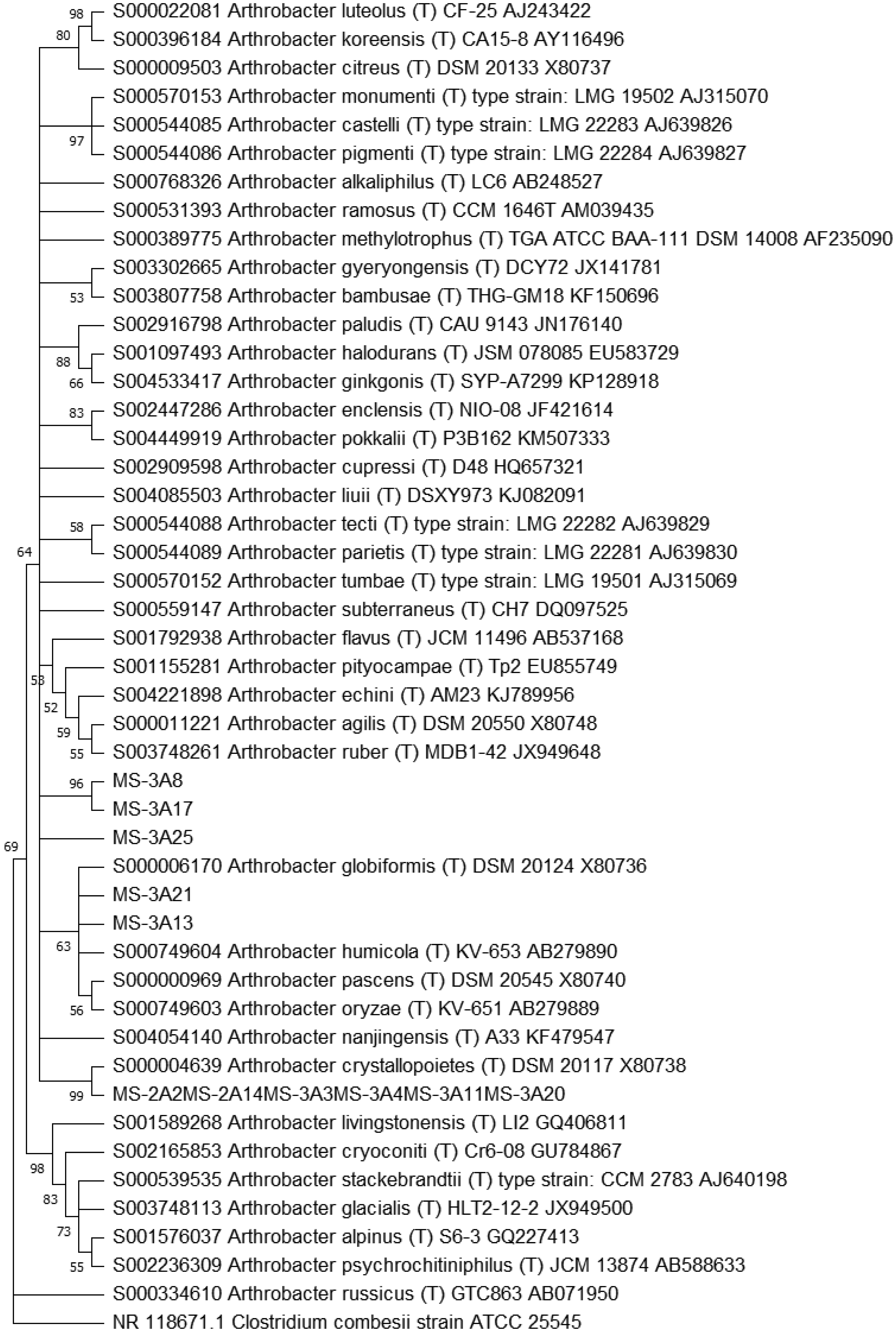
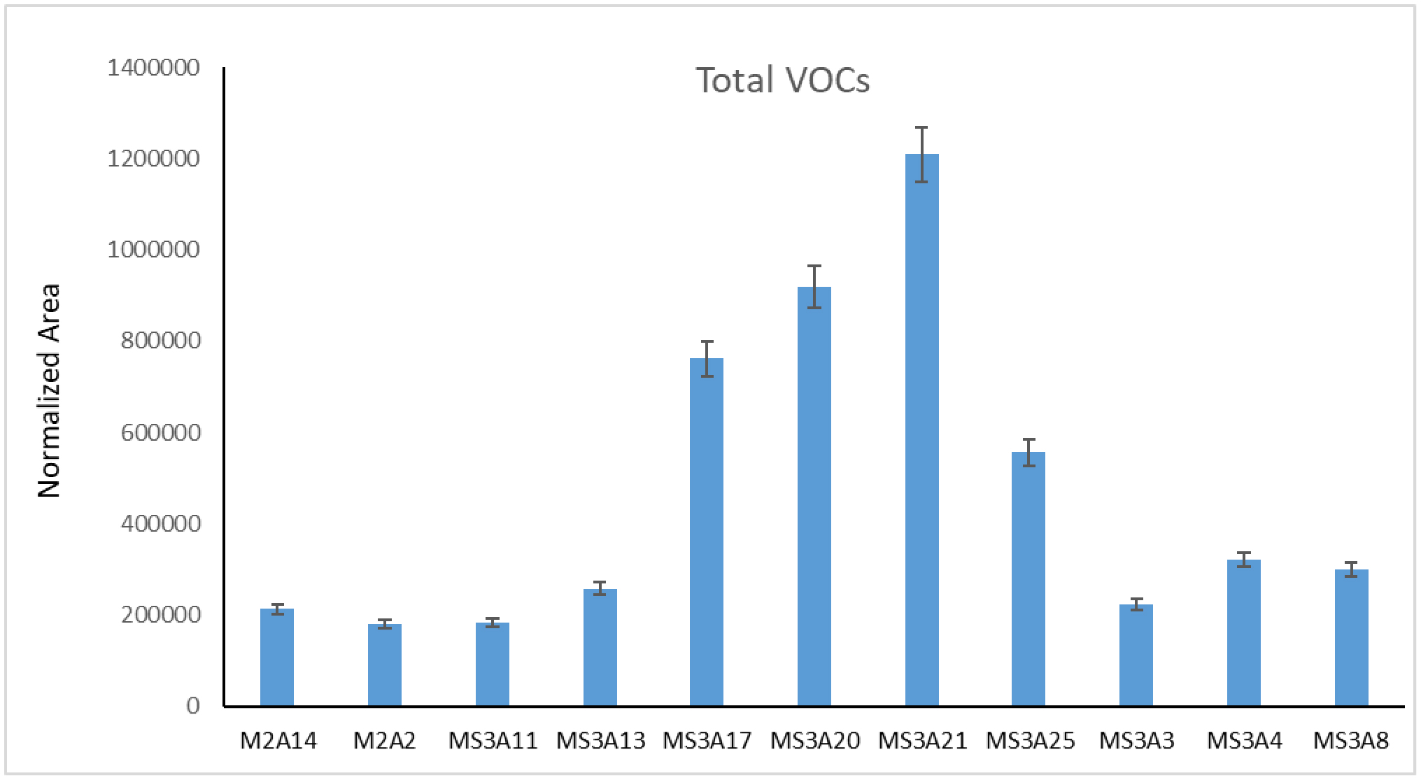
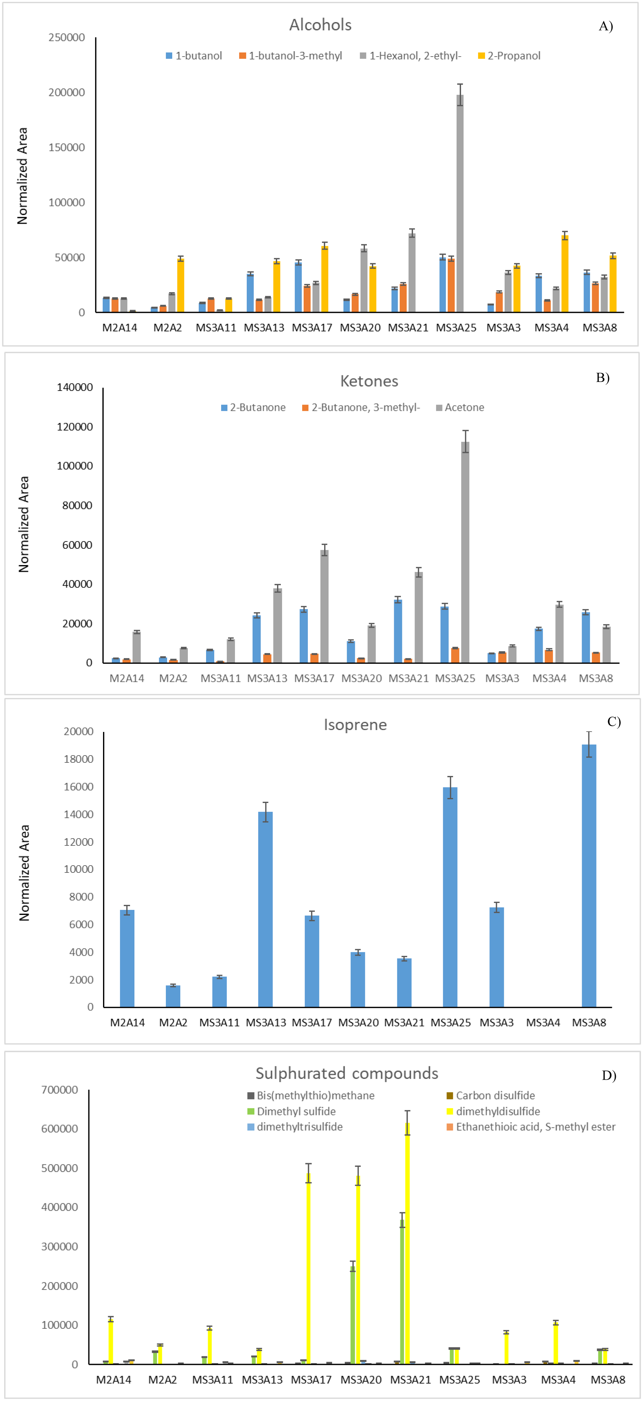
Desert soil hosts many microorganisms, whose activities are essential from an ecological viewpoint. Moreover, they are of great anthropic interest. The knowledge of extreme environments microbiomes may be beneficial for agriculture, technology, and human health. In this study, 11 Arthrobacter strains from topsoil samples collected from the Great Gobi A Strictly Protected Area in the Gobi Desert, were characterized by a combination of different techniques. The phylogenetic analysis, performed using their 16S rDNA sequences and the most similar Arthrobacter sequences found in databases, revealed that most of them were close to A. crystallopoietes, while others joined a sister group to the clade formed by A. humicola, A. pascens, and A. oryzae. The resistance of each strain to different antibiotics, heavy-metals, and NaCl was also tested as well as the inhibitory potential against human pathogens (i.e., Burkholderia ssp., Klebsiella pneumoniae, Pseudomonas aeruginosa, and Staphylococcus ssp.) via cross-streaking, to check the production of metabolites with antimicrobial activity. Data obtained revealed that all strains were resistant to heavy metals and were able to strongly interfere with the growth of many of the human pathogens tested. The volatile organic compounds (VOCs) profile of the 11 Arthrobacter strains was also analyzed. A total of 16 different metabolites were found, some of which were already known for having an inhibitory action against different Gram-positive and Gram-negative bacteria. Isolate MS-3A13, producing the highest quantity of VOCs, is the most efficient against Burkholderia cepacia complex (Bcc), K. pneumoniae, and coagulase-negative Staphylococci (CoNS) strains. This work highlights the importance of understanding microbial populations' phenotypical characteristics and dynamics in extreme environments to uncover the antimicrobial potential of new species and strains.
- Gobi Desert,
- Arthrobacter,
- inhibitory action,
- antibiotic resistance,
- VOCs
Citation: Alberto Bernacchi, Giulia Semenzato, Manuel di Mascolo, Sara Amata, Angela Bechini, Fabiola Berti, Carmela Calonico, Valentina Catania, Giovanni Emiliani, Antonia Esposito, Claudia Greco, Stefano Mocali, Nadia Mucci, Anna Padula, Antonio Palumbo Piccionello, Battogtokh Nasanbat, Gantulga Davaakhuu, Munkhtsetseg Bazarragchaa, Francesco Riga, Claudio Augugliaro, Anna Maria Puglia, Marco Zaccaroni, Fani Renato. Antibacterial activity of Arthrobacter strains isolated from Great Gobi A Strictly Protected Area, Mongolia[J]. AIMS Microbiology, 2024, 10(1): 161-186. doi: 10.3934/microbiol.2024009

Related Papers:

Abstract

Desert soil hosts many microorganisms, whose activities are essential from an ecological viewpoint. Moreover, they are of great anthropic interest. The knowledge of extreme environments microbiomes may be beneficial for agriculture, technology, and human health. In this study, 11 Arthrobacter strains from topsoil samples collected from the Great Gobi A Strictly Protected Area in the Gobi Desert, were characterized by a combination of different techniques. The phylogenetic analysis, performed using their 16S rDNA sequences and the most similar Arthrobacter sequences found in databases, revealed that most of them were close to A. crystallopoietes, while others joined a sister group to the clade formed by A. humicola, A. pascens, and A. oryzae. The resistance of each strain to different antibiotics, heavy-metals, and NaCl was also tested as well as the inhibitory potential against human pathogens (i.e., Burkholderia ssp., Klebsiella pneumoniae, Pseudomonas aeruginosa, and Staphylococcus ssp.) via cross-streaking, to check the production of metabolites with antimicrobial activity. Data obtained revealed that all strains were resistant to heavy metals and were able to strongly interfere with the growth of many of the human pathogens tested. The volatile organic compounds (VOCs) profile of the 11 Arthrobacter strains was also analyzed. A total of 16 different metabolites were found, some of which were already known for having an inhibitory action against different Gram-positive and Gram-negative bacteria. Isolate MS-3A13, producing the highest quantity of VOCs, is the most efficient against Burkholderia cepacia complex (Bcc), K. pneumoniae, and coagulase-negative Staphylococci (CoNS) strains. This work highlights the importance of understanding microbial populations' phenotypical characteristics and dynamics in extreme environments to uncover the antimicrobial potential of new species and strains.

Conflict of interest

Renato Fani is an editorial board member for AIMS Microbiology and was not involved in the editorial review or the decision to publish this article. All authors declare that there are no competing interests.

Author contributions

Conceptualization: Renato Fani, Giulia Semenzato, Marco Zaccaroni. Investigation: Alberto Bernacchi, Giulia Semenzato, Sara Amata, Antonia Esposito, Manuel di Mascolo, Fabiola Berti, Valentina Catania, Anna Padula. Visualization: Alberto Bernacchi, Renato Fani. Writing-Original Draft: Alberto Bernacchi, Giulia Semenzato, Renato Fani. Resources: Battogtoh Nasanbat, Gantulga Davaakhuu, Munkhtsetseg Bazarragchaa, Francesco Riga, Claudio Augugliaro, Marco Zaccaroni. Supervision: Anna Maria Puglia, Angela Bechini, Giovanni Emiliani, Stefano Mocali, Anna Padula, Marco Zaccaroni, Antonio Palumbo Piccionello. Writing-Review & Editing: Renato Fani, Marco Zaccaroni, Antonia Esposito, Giovanni Emiliani, Carmela Calonico, Angela Bechini, Giulia Semenzato, Alberto Bernacchi, Antonio Palumbo Piccionello, Anna Maria Puglia, Claudia Greco, Nadia Mucci, Anna Padula.

References

[1]	Jafari M, Tavili A, Panahi F, et al. (2018) Characteristics of arid and desert ecosystems. Reclamation of Arid Lands. Environmental Science and Engineering. Cham: Springer: 21-29. https://doi.org/10.1007/978-3-319-54828-9_2
[2]	Skujinš J (1984) Microbial ecology of desert soils. Advances in Microbial Ecology. Boston, MA: Springer: 49-91. https://doi.org/10.1007/978-1-4684-8989-7_2
[3]	Jafari M, Tavili A, Panahi F, et al. (2018) Reclamation of arid lands. Berlin/Heidelberg, Germany: Springer International Publishing. https://doi.org/10.1007/978-3-319-54828-9_2
[4]	Alsharif W, Saad MM, Hirt H (2020) Desert microbes for boosting sustainable agriculture in extreme environments. Front Microbiol 11: 1666. https://doi.org/10.3389/fmicb.2020.01666
[5]	Perera I, Subashchandrabose SR, Venkateswarlu K, et al. (2018) Consortia of cyanobacteria/microalgae and bacteria in desert soils: an underexplored microbiota. Appl Microbiol Biotechnol 102: 7351-7363. https://doi.org/10.1007/s00253-018-9192-1
[6]	Belnap J, Büdel B, Lange OL (2001) Biological soil crusts: characteristics and distribution. Biological Soil Crusts: Structure, Function, and Management. Ecological Studies. Berlin, Heidelberg: Springer: 3-30. https://doi.org/10.1007/978-3-642-56475-8_1
[7]	An S, Couteau C, Luo F, et al. (2013) Bacterial diversity of surface sand samples from the Gobi and Taklamaken deserts. Microb Ecol 66: 850-860. https://doi.org/10.1007/s00248-013-0276-2
[8]	Li SJ, Hua ZS, Huang LN, et al. (2014) Microbial communities evolve faster in extreme environments. Sci Rep 4: 6205. https://doi.org/10.1038/srep06205
[9]	Kaczensky P, Walzer C Wild camel training and collaring mission for the Great Gobi A Strictly Protected Area in Mongolia Wild camel training and collaring mission for the Great Gobi A Strictly Protected Area in Mongolia ‘Conservation of the Great Gobi Ecosystem and Its Umbrella Species Project’ Final report for UNDP for the short-term international expert contracts: 1. Data Processing and Analysis of collared wild camels 2. Wild camel satellite collaring and monitoring (2006). Available from: https://www.researchgate.net/profile/Chris-Walzer/publication/228483167_Wild_camel_training_and_collaring_mission_for_the_Great_Gobi_A_Strictly_Protected_Area_in_Mongolia/links/0fcfd50eebfeba1ab9000000/Wild-camel-training-and-collaring-mission-for-the-Great-Gobi-A-Strictly-Protected-Area-in-Mongolia.pdf
[10]	Shu WS, Huang LN (2022) Microbial diversity in extreme environments. Nat Rev Microbiol 20: 219-235. https://doi.org/10.1038/s41579-021-00648-y
[11]	Maida I, Bosi E, Fondi M, et al. (2015) Antimicrobial activity of Pseudoalteromonas strains isolated from the Ross Sea (Antarctica) versus Cystic Fibrosis opportunistic pathogens. Hydrobiologia 761: 443-457. https://doi.org/10.1007/s10750-015-2190-8
[12]	Tedesco P, Maida I, Palma Esposito F, et al. (2016) Antimicrobial activity of monoramnholipids produced by bacterial strains isolated from the Ross Sea (Antarctica). Mar Drugs 14: 83. https://doi.org/10.3390/md14050083
[13]	Papaleo MC, Fondi M, Maida I, et al. (2012) Sponge-associated microbial Antarctic communities exhibiting antimicrobial activity against Burkholderia cepacia complex bacteria. Biotechnol Adv 30: 272-293. https://doi.org/10.1016/j.biotechadv.2011.06.011
[14]	Romoli R, Papaleo MC, De Pascale D, et al. (2014) GC–MS volatolomic approach to study the antimicrobial activity of the antarctic bacterium Pseudoalteromonas sp. TB41. Metabolomics 10: 42-51. https://doi.org/10.1007/s11306-013-0549-2
[15]	Papaleo MC, Romoli R, Bartolucci G, et al. (2013) Bioactive volatile organic compounds from Antarctic (sponges) bacteria. New Biotechnol 30: 824-838. https://doi.org/10.1016/j.nbt.2013.03.011
[16]	Brown MG, Balkwill DL (2009) Antibiotic resistance in bacteria isolated from the deep terrestrial subsurface. Microb Ecol 57: 484-493. https://doi.org/10.1007/s00248-008-9431-6
[17]	Romero D, Traxler FM, Lòpez D, et al. (2011) Antibiotics as signal molecules. Chem Rev 111: 5492-5505. https://doi.org/10.1021/cr2000509
[18]	Delfino V., Calonico C., Nostro A. L., et al. (2021) Antibacterial activity of bacteria isolated from Phragmites australis against multidrug-resistant human pathogens. Future Microbiol 16: 291-303. https://doi.org/10.2217/fmb-2020-0244
[19]	Semenzato G, Del Duca S, Vassallo A, et al. (2023) Exploring the nexus between the composition of essential oil and the bacterial phytobiome associated with different compartments of the medicinal plants Origanum vulgare ssp. vulgare, O. vulgare ssp. hirtum, and O. heracleoticum. Ind Crops Prod 191. https://doi.org/10.1016/j.indcrop.2022.115997
[20]	Mori E, Liò P, Daly S, et al. (1999) Molecular nature of RAPD markers from Haemophilus influenzae Rd genome. Res Microbiol 150: 83-93. https://doi.org/10.1016/s0923-2508(99)80026-6
[21]	Edgar RC (2004) MUSCLE: Multiple sequence alignment with high accuracy and high throughput. Nucleic Acids Res 32: 1792-1797. https://doi.org/10.1093/nar/gkh340
[22]	Tamura K, Stecher G, Kumar S (2021) MEGA11: molecular evolutionary genetics analysis version 11. Mol Biol Evol 38: 3022-3027. https://doi.org/10.1093/molbev/msab120
[23]	Polito G, Semenzato G, Del Duca S, et al. (2022) Endophytic bacteria and essential oil from Origanum vulgare ssp. vulgare share some vocs with an antibacterial activity. Microorganisms 10. https://doi.org/10.3390/microorganisms10071424
[24]	Chiellini C, Maida I, Emiliani G, et al. (2014) Endophytic and rhizospheric bacterial communities isolated from the medicinal plants Echinacea purpurea and Echinacea angustifolia. Int Microbiol 17: 165-174. https://doi.org/10.2436/20.1501.01.219
[25]	Semenzato G, Del Duca S, Vassallo A, et al. (2023) Exploring the nexus between the composition of essential oil and the bacterial phytobiome associated with different compartments of the medicinal plants Origanum vulgare ssp. vulgare, O. vulgare ssp. hirtum, and O. heracleoticum. Ind Crops Prod 191. https://doi.org/10.1016/j.indcrop.2022.115997
[26]	Semenzato G, Del Duca S, Vassallo A, et al. (2023) Genomic, molecular, and phenotypic characterization of Arthrobacter sp. OVS8, an Endophytic bacterium isolated from and contributing to the bioactive compound content of the essential oil of the medicinal plant Origanum vulgare L. Int J Mol Sci 24: 4845. https://doi.org/10.3390/ijms24054845
[27]	Shu WS, Huang LN (2022) Microbial diversity in extreme environments. Nat Rev Microbiol 20: 219-235. https://doi.org/10.1038/s41579-021-00648-y
[28]	Roy P, Kumar A (2020) Chapter 1-Arthrobacter. Beneficial Microbes in Agro-Ecology.Academic Press: 3-11. https://doi.org/10.1016/B978-0-12-823414-3.00001-0
[29]	Boylen1 CW (1973) Survival of Arthrobacter crystallopoietes during prolonged periods of extreme desiccation. J Bacteriol 113. https://doi.org/10.1128/jb.113.1.33-37.1973
[30]	Joshi MN, Pandit AS, Sharma A, et al. (2013) Draft genome sequence of Arthrobacter crystallopoietes strain BAB-32, revealing genes for bioremediation. Genome Announc 1. https://doi.org/10.1128/genomeA.00452-13
[31]	Keddie RM, Jones D (1981) Saprophytic, aerobic coryneform bacteria. Prokaryotes 2: 1838-1878.
[32]	Camargo FA, Okeke BC, Bento FM, et al. (2003) In vitro reduction of hexavalent chromium by a cell-free extract of Bacillus sp. ES 29 stimulated by Cu2+. Appl Microbiol Biotechnol 62: 569-573. https://doi.org/10.1007/s00253-003-1291-x
[33]	Marques CR, Caetano AL, Haller A, et al. (2014) Toxicity screening of soils from different mine areas-A contribution to track the sensitivity and variability of Arthrobacter globiformis assay. J Hazard Mater 274: 331-341. https://doi.org/10.1016/j.jhazmat.2014.03.066
[34]	Sekiguchi Y, Makita H, Yamamura A, et al. (2004) A thermostable histamine oxidase from Arthrobacter crystallopoietes KAIT-B-007. J Biosci Bioeng 97: 104-110. https://doi.org/10.1016/S1389-1723(04)70176-0
[35]	Kumar S, Suyal DC, Yadav A, et al. (2019) Microbial diversity and soil physiochemical characteristic of higher altitude. PLoS One 14. https://doi.org/10.1371/journal.pone.0213844
[36]	Heuer H, Smalla K (2012) Plasmids foster diversification and adaptation of bacterial populations in soil. FEMS Microbiol Rev 36: 1083-1104. https://doi.org/10.1111/j.1574-6976.2012.00337.x
[37]	Naidoo Y, Valverde A, Cason ED, et al. (2020) A clinically important, plasmid-borne antibiotic resistance gene (β-lactamase TEM-116) present in desert soils. Sci Total Environ 719: 137497. https://doi.org/10.1016/j.scitotenv.2020.137497
[38]	Larsson DGJ, Flach CF (2022) Antibiotic resistance in the environment. Nat Rev Microbiol 20: 257-269. https://doi.org/10.1038/s41579-021-00649-x
[39]	Moloney MG (2016) Natural products as a source for novel antibiotics. Trends Pharmacol Sci 37: 689-701. https://doi.org/10.1016/j.tips.2016.05.001
[40]	Papazlatani C, Rousidou C, Katsoula A, et al. (2016) Assessment of the impact of the fumigant dimethyl disulfide on the dynamics of major fungal plant pathogens in greenhouse soils. Eur J Plant Pathol 146: 391-400. https://doi.org/10.1007/s10658-016-0926-6
[41]	Romoli R, Papaleo MC, de Pascale D, et al. (2011) Characterization of the volatile profile of Antarctic bacteria by using solid-phase microextraction-gas chromatography-mass spectrometry. JMS 46: 1051-1059. https://doi.org/10.1002/jms.1987
[42]	Effmert U, Kalderás J, Warnke R, et al. (2012) Volatile mediated interactions between bacteria and fungi in the soil. J Chem Ecol 38: 665-703. https://doi.org/10.1007/s10886-012-0135-5

microbiol-10-01-009-s001.pdf

Reader Comments

Your name:*

Email:*
© 2024 the Author(s), licensee AIMS Press. This is an open access article distributed under the terms of the Creative Commons Attribution License (http://creativecommons.org/licenses/by/4.0)