Exploring endophytes for <i>in vitro</i> synthesis of bioactive compounds similar to metabolites produced <i>in vivo</i> by host plants

Hemant Sharma; Arun Kumar Rai; Divakar Dahiya; Rajen Chettri; Poonam Singh Nigam; Hemant Sharma; Arun Kumar Rai; Divakar Dahiya; Rajen Chettri; Poonam Singh Nigam

doi:10.3934/microbiol.2021012

AIMS Microbiology

2021, Volume 7, Issue 2: 175-199. doi: 10.3934/microbiol.2021012

Previous Article Next Article

Mini review Special Issues

Exploring endophytes for in vitro synthesis of bioactive compounds similar to metabolites produced in vivo by host plants

1.
Department of Botany, Sikkim University, 6^th Mile Tadong, Gangtok, Sikkim, India
2.
School of Human Sciences, London Metropolitan University, Holloway Road, London, UK
3.
Department of Botany, Sikkim Government Science College, Chakung, Sikkim, India
4.
Biomedical Sciences Research Institute, Ulster University, Coleraine, Northern Ireland, UK

Received: 04 February 2021 Accepted: 19 May 2021 Published: 26 May 2021

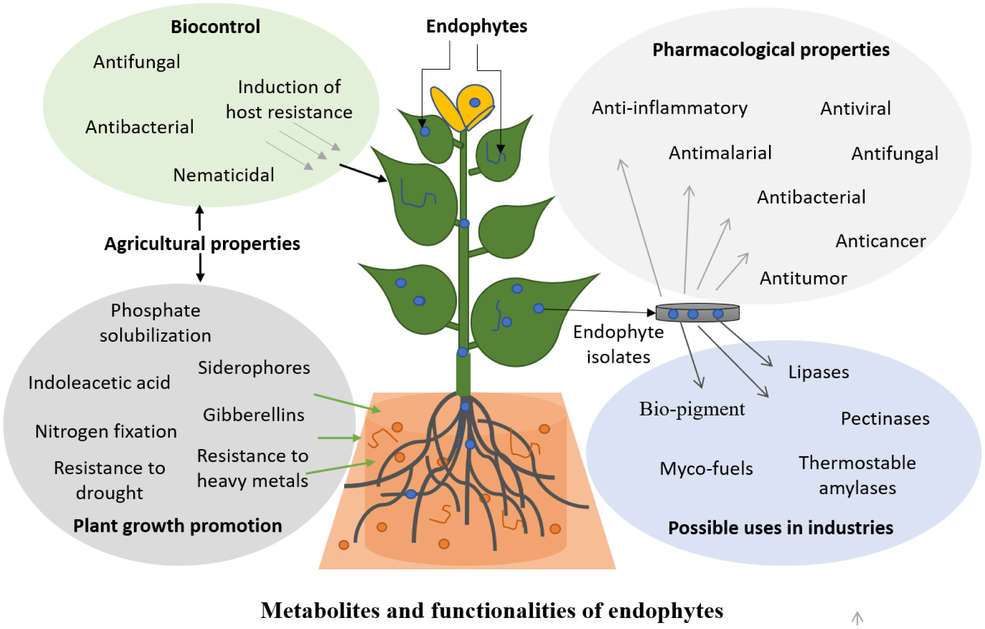
Endophytes represent microorganisms residing within plant tissues without typically causing any adverse effect to the plants for considerable part of their life cycle and are primarily known for their beneficial role to their host-plant. These microorganisms can in vitro synthesize secondary metabolites similar to metabolites produced in vivo by their host plants. If microorganisms are isolated from certain plants, there is undoubtedly a strong possibility of obtaining beneficial endophytes strains producing host-specific secondary metabolites for their potential applications in sustainable agriculture, pharmaceuticals and other industrial sectors. Few products derived from endophytes are being used for cultivating resilient crops and developing non-toxic feeds for livestock. Our better understanding of the complex relationship between endophytes and their host will immensely improve the possibility to explore their unlimited functionalities. Successful production of host-secondary metabolites by endophytes at commercial scale might progressively eliminate our direct dependence on high-valued vulnerable plants, thus paving a viable way for utilizing plant resources in a sustainable way.
- Endophytes,
- biomolecules,
- secondary-metabolites
Citation: Hemant Sharma, Arun Kumar Rai, Divakar Dahiya, Rajen Chettri, Poonam Singh Nigam. Exploring endophytes for in vitro synthesis of bioactive compounds similar to metabolites produced in vivo by host plants[J]. AIMS Microbiology, 2021, 7(2): 175-199. doi: 10.3934/microbiol.2021012

Related Papers:

Abstract

Endophytes represent microorganisms residing within plant tissues without typically causing any adverse effect to the plants for considerable part of their life cycle and are primarily known for their beneficial role to their host-plant. These microorganisms can in vitro synthesize secondary metabolites similar to metabolites produced in vivo by their host plants. If microorganisms are isolated from certain plants, there is undoubtedly a strong possibility of obtaining beneficial endophytes strains producing host-specific secondary metabolites for their potential applications in sustainable agriculture, pharmaceuticals and other industrial sectors. Few products derived from endophytes are being used for cultivating resilient crops and developing non-toxic feeds for livestock. Our better understanding of the complex relationship between endophytes and their host will immensely improve the possibility to explore their unlimited functionalities. Successful production of host-secondary metabolites by endophytes at commercial scale might progressively eliminate our direct dependence on high-valued vulnerable plants, thus paving a viable way for utilizing plant resources in a sustainable way.

Funding

This research did not receive any specific grant from funding agencies in the public, commercial, or not-for-profit sectors.

Conflict of interest

All authors declare no conflicts of interest in this review article.

References

[1]	Saikkonen K, Faeth SH, Helander M, et al. (1998) Fungal endophytes: a continuum of interactions with host plants. Annu Rev Ecol Syst 29: 319-343. doi: 10.1146/annurev.ecolsys.29.1.319
[2]	Patwardhan B, Warude D, Pushpangadan P, et al. (2005) Ayurveda and traditional Chinese medicine: A comparative overview. Evidence-based Complement Altern Med 2: 465-473. doi: 10.1093/ecam/neh140
[3]	Sigerist HE (1987) A history of medicine: Early Greek, Hindu, and Persian medicine New York: Oxford University Press.
[4]	Sofowora A (1996) Research on medicinal plants and traditional medicine in Africa. J Altern Complement Med 2: 365-372. doi: 10.1089/acm.1996.2.365
[5]	Verma S, Singh S (2008) Current and future status of herbal medicines. Vet World 2: 347. doi: 10.5455/vetworld.2008.347-350
[6]	Yuan H, Ma Q, Ye L, et al. (2016) The traditional medicine and modern medicine from natural products. Molecules 21: 559. doi: 10.3390/molecules21050559
[7]	Mendelsohn R, Balick MJ (1995) The value of undiscovered pharmaceuticals in tropical forests. Econ Bot 49: 223-228. doi: 10.1007/BF02862929
[8]	Hamilton AC (2004) Medicinal plants, conservation and livelihoods. Biodivers Conserv 13: 1477-1517. doi: 10.1023/B:BIOC.0000021333.23413.42
[9]	WHO (2002) WHO Traditional Medicine Strategy Geneva: World Health Organization.
[10]	Ten Kate K, Laird SA (2002) The commercial use of biodiversity: access to genetic resources and benefit-sharing London: Earthscan.
[11]	Yarnell E, Abascal K (2002) Dilemmas of traditional botanical research. HerbalGram 55: 46-54.
[12]	Abebe W (2002) Herbal medication: potential for adverse interactions with analgesic drugs. J Clin Pharm Ther 27: 391-401. doi: 10.1046/j.1365-2710.2002.00444.x
[13]	Allkin B (2017) Useful plants–Medicines: At least 28,187 plant species are currently recorded as being of medicinal use London (UK): Royal Botanic Gardens, Kew.
[14]	Wani ZA, Ashraf N, Mohiuddin T, et al. (2015) Plant-endophyte symbiosis, an ecological perspective. Appl Microbiol Biotechnol 99: 2955-2965. doi: 10.1007/s00253-015-6487-3
[15]	Mostert L, Crous PW, Petrini O (2000) Endophytic fungi associated with shoots and leaves of Vitis vinifera, with specific reference to the Phomopsis viticola complex. Sydowia 52: 46-58.
[16]	Rodriguez RJ, White JF, Arnold AE, et al. (2009) Fungal endophytes: diversity and functional roles. New Phytol 182: 314-330. doi: 10.1111/j.1469-8137.2009.02773.x
[17]	Rajamanikyam M, Vadlapudi V, Amanchy R, et al. (2017) Endophytic fungi as novel resources of natural therapeutics. Brazilian Arch Biol Technol 60: 451-454. doi: 10.1590/1678-4324-2017160542
[18]	Le Cocq K, Gurr SJ, Hirsch PR, et al. (2017) Exploitation of endophytes for sustainable agricultural intensification. Mol Plant Pathol 18: 469-473. doi: 10.1111/mpp.12483
[19]	Sudheep NM, Marwal A, Lakra N, et al. (2017) Plant-microbe interactions in agro-ecological perspectives Singapore: Springer Singapore.
[20]	Bacon CW, White JF (2000) Physiological adaptations in the evolution of endophytism in the Clavicipitaceae. Microb endophytes 251-276. doi: 10.1201/9781482277302-13
[21]	Wang H, Hyde KD, Soytong K, et al. (2008) Fungal diversity on fallen leaves of Ficus in northern Thailand. J Zhejiang Univ Sci B 9: 835-841. doi: 10.1631/jzus.B0860005
[22]	Bacon CW, Porter JK, Robbins JD (1975) Toxicity and occurrence of Balansia on grasses from toxic fescue pastures. Appl Microbiol 29: 553-556. doi: 10.1128/am.29.4.553-556.1975
[23]	Nair DN, Padmavathy S (2014) Impact of endophytic microorganisms on plants, environment and humans. Sci World J 2014: 1-11. doi: 10.1155/2014/250693
[24]	Arnold A, Maynard Z, Gilbert G, et al. (2000) Are tropical fungal endophytes hyperdiverse? Ecol Lett 3: 267-274. doi: 10.1046/j.1461-0248.2000.00159.x
[25]	Potshangbam M, Devi SI, Sahoo D, et al. (2017) Functional characterization of endophytic fungal community associated with Oryza sativa L. and Zea mays L. Front Microbiol 8: 1-15. doi: 10.3389/fmicb.2017.00325
[26]	Lu Y, Chen C, Chen H, et al. (2012) Isolation and identification of endophytic fungi from Actinidia macrosperma and investigation of their bioactivities. Evidence-Based Complement Altern Med 2012: 1-8.
[27]	Sun X, Guo L (2015) Endophytic fungal diversity: review of traditional and molecular techniques. Mycology 3: 1203.
[28]	Suhandono S, Kusumawardhani MK, Aditiawati P (2016) Isolation and molecular identification of endophytic bacteria from Rambutan fruits (Nephelium lappaceum L.) cultivar Binjai. HAYATI J Biosci 23: 39-44. doi: 10.1016/j.hjb.2016.01.005
[29]	Hiroyuki K, Satoshi T, Shun-ichi T, et al. (1989) New fungitoxic Sesquiterpenoids, Chokols A-G, from stromata of Epichloe typhina and the absolute configuration of Chokol E. Agric Biol Chem 53: 789-796. doi: 10.1080/00021369.1989.10869341
[30]	Sahai AS, Manocha MS (1993) Chitinases of fungi and plants: their involvement in morphogenesis and host-parasite interaction. FEMS Microbiol Rev 11: 317-338. doi: 10.1111/j.1574-6976.1993.tb00004.x
[31]	Pleban S, Chernin L, Chet I (1997) Chitinolytic activity of an endophytic strain of Bacillus cereus. Lett Appl Microbiol 25: 284-288. doi: 10.1046/j.1472-765X.1997.00224.x
[32]	Pennell C, Rolston M, De Bonth A, et al. (2010) Development of a bird-deterrent fungal endophyte in turf tall fescue. New Zeal J Agric Res 53: 145-150. doi: 10.1080/00288231003777681
[33]	Rajulu MBG, Thirunavukkarasu N, Suryanarayanan TS, et al. (2011) Chitinolytic enzymes from endophytic fungi. Fungal Divers 47: 43-53. doi: 10.1007/s13225-010-0071-z
[34]	Zheng YK, Miao CP, Chen HH, et al. (2017) Endophytic fungi harbored in Panax notoginseng: Diversity and potential as biological control agents against host plant pathogens of root-rot disease. J Ginseng Res 41: 353-360. doi: 10.1016/j.jgr.2016.07.005
[35]	Cairney JWG, Burke RM (1998) Extracellular enzyme activities of the ericoid mycorrhizal endophyte Hymenoscyphus ericae (Read) Korf & Kernan: their likely roles in decomposition of dead plant tissue in soil. Plant Soil 205: 181-192. doi: 10.1023/A:1004376731209
[36]	Lu H, Zou WX, Meng JC, et al. (2000) New bioactive metabolites produced by Colletotrichum sp., an endophytic fungus in Artemisia annua. Plant Sci 151: 67-73. doi: 10.1016/S0168-9452(99)00199-5
[37]	Ahmad N, Hamayun M, Khan SA, et al. (2010) Gibberellin-producing endophytic fungi isolated from Monochoria vaginalis. J Microbiol Biotechnol 20: 1744-1749.
[38]	Forchetti G, Masciarelli O, Alemano S, et al. (2007) Endophytic bacteria in sunflower (Helianthus annuus L.): isolation, characterization, and production of jasmonates and abscisic acid in culture medium. Appl Microbiol Biotechnol 76: 1145-1152. doi: 10.1007/s00253-007-1077-7
[39]	Shahabivand S, Maivan HZ, Goltapeh EM, et al. (2012) The effects of root endophyte and arbuscular mycorrhizal fungi on growth and cadmium accumulation in wheat under cadmium toxicity. Plant Physiol Biochem 60: 53-58. doi: 10.1016/j.plaphy.2012.07.018
[40]	Yanni YG, Dazzo FB (2010) Enhancement of rice production using endophytic strains of Rhizobium leguminosarum bv. trifolii in extensive field inoculation trials within the Egypt Nile delta. Plant Soil 336: 129-142. doi: 10.1007/s11104-010-0454-7
[41]	Zhang Y, Kang X, Liu H, et al. (2018) Endophytes isolated from ginger rhizome exhibit growth promoting potential for Zea mays. Arch Agron Soil Sci 64: 1302-1314. doi: 10.1080/03650340.2018.1430892
[42]	Waqas M, Khan AL, Kang S-M, et al. (2014) Phytohormone-producing fungal endophytes and hardwood-derived biochar interact to ameliorate heavy metal stress in soybeans. Biol Fertil Soils 50: 1155-1167. doi: 10.1007/s00374-014-0937-4
[43]	Yamaji K, Watanabe Y, Masuya H, et al. (2016) Root fungal endophytes enhance heavy-metal stress tolerance of Clethra barbinervis growing naturally at mining sites via growth enhancement, promotion of nutrient uptake and decrease of heavy-metal concentration. PLoS One 11: 1-15.
[44]	Maggini V, Mengoni A, Gallo ER, et al. (2019) Tissue specificity and differential effects on in vitro plant growth of single bacterial endophytes isolated from the roots, leaves and rhizospheric soil of Echinacea purpurea. BMC Plant Biol 19: 284. doi: 10.1186/s12870-019-1890-z
[45]	Abdelshafy Mohamad OA, Ma J-B, Liu Y-H, et al. (2020) Beneficial endophytic bacterial populations associated with medicinal plant Thymus vulgaris alleviate salt stress and confer resistance to Fusarium oxysporum. Front Plant Sci 11: 1-17. doi: 10.3389/fpls.2020.00047
[46]	Castronovo LM, Calonico C, Ascrizzi R, et al. (2020) The cultivable bacterial microbiota associated to the medicinal plant Origanum vulgare L.: from antibiotic resistance to growth-inhibitory properties. Front Microbiol 11: 1-17. doi: 10.3389/fmicb.2020.00862
[47]	Pereira SIA, Monteiro C, Vega AL, et al. (2016) Endophytic culturable bacteria colonizing Lavandula dentata L. plants: Isolation, characterization and evaluation of their plant growth-promoting activities. Ecol Eng 87: 91-97. doi: 10.1016/j.ecoleng.2015.11.033
[48]	Snook ME, Mitchell T, Hinton DM, et al. (2009) Isolation and characterization of Leu 7-surfactin from the endophytic Bbacterium Bacillus mojavensis RRC 101, a biocontrol agent for Fusarium verticillioides. J Agric Food Chem 57: 4287-4292. doi: 10.1021/jf900164h
[49]	Nyambura Ngamau C (2012) Isolation and identification of endophytic bacteria of bananas (Musa spp.) in Kenya and their potential as biofertilizers for sustainable banana production. African J Microbiol Res 6: 6414-6422. doi: 10.5897/AJMR12.1170
[50]	Rungin S, Indananda C, Suttiviriya P, et al. (2012) Plant growth enhancing effects by a siderophore-producing endophytic streptomycete isolated from a Thai jasmine rice plant (Oryza sativa L. cv. KDML105). Antonie Van Leeuwenhoek 102: 463-472. doi: 10.1007/s10482-012-9778-z
[51]	Naveed M, Mitter B, Yousaf S, et al. (2013) The endophyte Enterobacter sp. FD17: A maize growth enhancer selected based on rigorous testing of plant beneficial traits and colonization characteristics. Biol Fertil Soils 50: 249-262. doi: 10.1007/s00374-013-0854-y
[52]	Hiroyuki K, Satoshi T, Shun-ichi T, et al. (1989) New fungitoxic sesquiterpenoids, chokols A-G, from stromata of Epichloe typhina and the absolute configuration of chokol E. Agric Biol Chem 53: 789-796. doi: 10.1080/00021369.1989.10869341
[53]	Findlay JA, Li G, Johnson JA (1997) Bioactive compounds from an endophytic fungus from eastern larch (Larix laricina) needles. Can J Chem 75: 716-719. doi: 10.1139/v97-086
[54]	Wakelin SA, Warren RA, Harvey PR, et al. (2004) Phosphate solubilization by Penicillium spp. closely associated with wheat roots. Biol Fertil Soils 40: 36-43. doi: 10.1007/s00374-004-0750-6
[55]	Schwarz M, Köpcke B, Weber RWS, et al. (2004) 3-Hydroxypropionic acid as a nematicidal principle in endophytic fungi. Phytochemistry 65: 2239-2245. doi: 10.1016/j.phytochem.2004.06.035
[56]	Strobel G (2006) Harnessing endophytes for industrial microbiology. Curr Opin Microbiol 9: 240-244. doi: 10.1016/j.mib.2006.04.001
[57]	Kuldau G, Bacon C (2008) Clavicipitaceous endophytes: Their ability to enhance resistance of grasses to multiple stresses. Biol Control 46: 57-71. doi: 10.1016/j.biocontrol.2008.01.023
[58]	Kajula M, Tejesvi MV, Kolehmainen S, et al. (2010) The siderophore ferricrocin produced by specific foliar endophytic fungi in vitro. Fungal Biol 114: 248-254. doi: 10.1016/j.funbio.2010.01.004
[59]	Tomsheck AR, Strobel GA, Booth E, et al. (2010) Hypoxylon sp., an endophyte of Persea indica, producing 1,8-Cineole and other bioactive volatiles with fuel potential. Microb Ecol 60: 903-914. doi: 10.1007/s00248-010-9759-6
[60]	Nath R, Sharma GD, Barooah M (2012) Efficiency of tricalcium phosphate solubilization by two different endophytic Penicillium sp. isolated from tea (Camellia sinensis L.). Eur J Exp Biol 2: 1354-1358.
[61]	Waqas M, Khan AL, Kamran M, et al. (2012) Endophytic fungi produce gibberellins and indoleacetic acid and promotes host-plant growth during stress. Molecules 17: 10754-10773. doi: 10.3390/molecules170910754
[62]	Kedar A, Rathod D, Yadav A, et al. (2014) Endophytic Phoma sp. isolated from medicinal plants promote the growth of Zea mays. Nusant Biosci 6: 132-139.
[63]	Shentu X, Zhan X, Ma Z, et al. (2014) Antifungal activity of metabolites of the endophytic fungus Trichoderma brevicompactum from garlic. Brazilian J Microbiol 45: 248-254. doi: 10.1590/S1517-83822014005000036
[64]	Abraham S, Basukriadi A, Pawiroharsono S, et al. (2015) Insecticidal activity of ethyl acetate extracts from culture filtrates of mangrove fungal endophytes. Mycobiology 43: 137-149. doi: 10.5941/MYCO.2015.43.2.137
[65]	Xin G, Glawe D, Doty SL (2009) Characterization of three endophytic, indole-3-acetic acid-producing yeasts occurring in Populus trees. Mycol Res 113: 973-980. doi: 10.1016/j.mycres.2009.06.001
[66]	Pye CR, Bertin MJ, Lokey RS, et al. (2017) Retrospective analysis of natural products provides insights for future discovery trends. Proc Natl Acad Sci 114: 5601-5606. doi: 10.1073/pnas.1614680114
[67]	Sen S, Chakraborty R (2017) Revival, modernization and integration of Indian traditional herbal medicine in clinical practice: Importance, challenges and future. J Tradit Complement Med 7: 234-244. doi: 10.1016/j.jtcme.2016.05.006
[68]	Romano G, Costantini M, Sansone C, et al. (2017) Marine microorganisms as a promising and sustainable source of bioactive molecules. Mar Environ Res 128: 58-69. doi: 10.1016/j.marenvres.2016.05.002
[69]	Matsumoto A, Takahashi Y (2017) Endophytic actinomycetes: promising source of novel bioactive compounds. J Antibiot (Tokyo) 70: 514-519. doi: 10.1038/ja.2017.20
[70]	Staniek A, Woerdenbag HJ, Kayser O (2008) Endophytes: Exploiting biodiversity for the improvement of natural product-based drug discovery. J Plant Interact 3: 75-93. doi: 10.1080/17429140801886293
[71]	Jin Z, Gao L, Zhang L, et al. (2017) Antimicrobial activity of saponins produced by two novel endophytic fungi from Panax notoginseng. Nat Prod Res 31: 2700-2703. doi: 10.1080/14786419.2017.1292265
[72]	Horn WS, Simmonds MSJ, Schwartz RE, et al. (1995) Phomopsichalasin, a novel antimicrobial agent from an endophytic Phomopsis sp. Tetrahedron 51: 3969-3978. doi: 10.1016/0040-4020(95)00139-Y
[73]	Liu JY, Song YC, Zhang Z, et al. (2004) Aspergillus fumigatus CY018, an endophytic fungus in Cynodon dactylon as a versatile producer of new and bioactive metabolites. J Biotechnol 114: 279-287. doi: 10.1016/j.jbiotec.2004.07.008
[74]	Kongsaeree P, Prabpai S, Sriubolmas N, et al. (2003) Antimalarial dihydroisocoumarins produced by Geotrichum sp., an endophytic fungus of Crassocephalum crepidioides. J Nat Prod 66: 709-711. doi: 10.1021/np0205598
[75]	Wang FW, Jiao RH, Cheng AB, et al. (2007) Antimicrobial potentials of endophytic fungi residing in Quercus variabilis and brefeldin A obtained from Cladosporium sp. World J Microbiol Biotechnol 23: 79-83. doi: 10.1007/s11274-006-9195-4
[76]	Eze P, Ojimba N, Abonyi D, et al. (2018) Antimicrobial activity of metabolites of an endophytic fungus isolated from the leaves of Citrus jambhiri (Rutaceae). Trop J Nat Prod Res 2: 145-149. doi: 10.26538/tjnpr/v2i3.9
[77]	Hoffman AM, Mayer SG, Strobel GA, et al. (2008) Purification, identification and activity of phomodione, a furandione from an endophytic Phoma species. Phytochemistry 69: 1049-1056. doi: 10.1016/j.phytochem.2007.10.031
[78]	Stierle A, Strobel G, Stierle D (1993) Taxol and taxane production by Taxomyces andreanae, an endophytic fungus of Pacific yew. Science (80-) 260: 214-216. doi: 10.1126/science.8097061
[79]	Chakravarthi BVSK, Das P, Surendranath K, et al. (2008) Production of paclitaxel by Fusarium solani isolated from Taxus celebica. J Biosci 33: 259-267. doi: 10.1007/s12038-008-0043-6
[80]	Kusari S, Lamshöft M, Spiteller M (2009) Aspergillus fumigatus Fresenius, an endophytic fungus from Juniperus communis L. Horstmann as a novel source of the anticancer pro-drug deoxypodophyllotoxin. J Appl Microbiol 107: 1019-1030. doi: 10.1111/j.1365-2672.2009.04285.x
[81]	Kusari S, Lamshöft M, Zühlke S, et al. (2008) An endophytic fungus from Hypericum perforatum that produces hypericin. J Nat Prod 71: 159-162. doi: 10.1021/np070669k
[82]	Parthasarathy R, Sathiyabama M (2015) Lovastatin-producing endophytic fungus isolated from a medicinal plant Solanum xanthocarpum. Nat Prod Res 29: 2282-2286. doi: 10.1080/14786419.2015.1016938
[83]	Ding L, Münch J, Goerls H, et al. (2010) Xiamycin, a pentacyclic indolosesquiterpene with selective anti-HIV activity from a bacterial mangrove endophyte. Bioorganic Med Chem Lett 20: 6685-6687. doi: 10.1016/j.bmcl.2010.09.010
[84]	Bhore S, Preveena J, Kandasamy K (2013) Isolation and identification of bacterial endophytes from pharmaceutical agarwood-producing Aquilaria species. Pharmacognosy Res 5: 134. doi: 10.4103/0974-8490.110545
[85]	Strobel GA, Miller RV, Martinez-Miller C, et al. (1999) Cryptocandin, a potent antimycotic from the endophytic fungus Cryptosporiopsis cf. quercina. Microbiology 145: 1919-1926. doi: 10.1099/13500872-145-8-1919
[86]	Aly AH, Edrada-Ebel RA, Wray V, et al. (2008) Bioactive metabolites from the endophytic fungus Ampelomyces sp. isolated from the medicinal plant Urospermum picroides. Phytochemistry 69: 1716-1725. doi: 10.1016/j.phytochem.2008.02.013
[87]	Huang Z, Cai X, Shao C, et al. (2008) Chemistry and weak antimicrobial activities of phomopsins produced by mangrove endophytic fungus Phomopsis sp. ZSU-H76. Phytochemistry 69: 1604-1608. doi: 10.1016/j.phytochem.2008.02.002
[88]	Gogoi DK, Deka Boruah HP, Saikia R, et al. (2008) Optimization of process parameters for improved production of bioactive metabolite by a novel endophytic fungus Fusarium sp. DF2 isolated from Taxus wallichiana of North East India. World J Microbiol Biotechnol 24: 79-87. doi: 10.1007/s11274-007-9442-3
[89]	Adelin E, Servy C, Cortial S, et al. (2011) Isolation, structure elucidation and biological activity of metabolites from Sch-642305-producing endophytic fungus Phomopsis sp. CMU-LMA. Phytochemistry 72: 2406-2412. doi: 10.1016/j.phytochem.2011.08.010
[90]	Nithya K, Muthumary J (2011) Bioactive metabolite produced by Phomopsis sp., an endophytic fungus in Allamanda cathartica Linn. Recent Res Sci Technol .
[91]	Tayung K, Barik BP, Jha DK, et al. (2011) Identification and characterization of antimicrobial metabolite from an endophytic fungus, Fusarium solani isolated from bark of Himalayan yew. Mycosphere 2: 203-213.
[92]	Zhang G, Sun S, Zhu T, et al. (2011) Antiviral isoindolone derivatives from an endophytic fungus Emericella sp. associated with Aegiceras corniculatum. Phytochemistry 72: 1436-1442. doi: 10.1016/j.phytochem.2011.04.014
[93]	Ai W, Wei X, Lin X, et al. (2014) Guignardins A-F, spirodioxynaphthalenes from the endophytic fungus Guignardia sp. KcF8 as a new class of PTP1B and SIRT1 inhibitors. Tetrahedron 70: 5806-5814. doi: 10.1016/j.tet.2014.06.041
[94]	Cui L, Wu S, Zhao C, et al. (2016) Microbial conversion of major ginsenosides in ginseng total saponins by Platycodon grandiflorum endophytes. J Ginseng Res 40: 366-374. doi: 10.1016/j.jgr.2015.11.004
[95]	Sakiyama CCH, Paula EM, Pereira PC, et al. (2001) Characterization of pectin lyase produced by an endophytic strain isolated from coffee cherries. Lett Appl Microbiol 33: 117-121. doi: 10.1046/j.1472-765x.2001.00961.x
[96]	Stamford TL, Stamford N., Coelho LCB, et al. (2001) Production and characterization of a thermostable α-amylase from Nocardiopsis sp. endophyte of yam bean. Bioresour Technol 76: 137-141. doi: 10.1016/S0960-8524(00)00089-4
[97]	Stamford TLM, Stamford NP, Coelho LCBB, et al. (2002) Production and characterization of a thermostable glucoamylase from Streptosporangium sp. endophyte of maize leaves. Bioresour Technol 83: 105-109. doi: 10.1016/S0960-8524(01)00206-1
[98]	Dorra G, Ines K, Imen BS, et al. (2018) Purification and characterization of a novel high molecular weight alkaline protease produced by an endophytic Bacillus halotolerans strain CT2. Int J Biol Macromol 111: 342-351. doi: 10.1016/j.ijbiomac.2018.01.024
[99]	Choi YW, Hodgkiss IJ, Hyde KD (2005) Enzyme production by endophytes of Brucea javanica. J Agric Technol 55-66.
[100]	Peng XW, Chen HZ (2007) Microbial oil accumulation and cellulase secretion of the endophytic fungi from oleaginous plants. Ann Microbiol 57: 239-242. doi: 10.1007/BF03175213
[101]	Strobel GA, Knighton B, Kluck K, et al. (2008) The production of myco-diesel hydrocarbons and their derivatives by the endophytic fungus Gliocladiurn roseum (NRRL 50072). Microbiology 154: 3319-3328. doi: 10.1099/mic.0.2008/022186-0
[102]	Russell JR, Huang J, Anand P, et al. (2011) Biodegradation of polyester polyurethane by endophytic fungi. Appl Environ Microbiol 77: 6076-6084. doi: 10.1128/AEM.00521-11
[103]	Defranceschi Oliveira AC, Farion Watanabe FM, Coelho Vargas JV, et al. (2012) Production of methyl oleate with a lipase from an endophytic yeast isolated from castor leaves. Biocatal Agric Biotechnol 1: 295-300. doi: 10.1016/j.bcab.2012.06.004
[104]	Zaferanloo B, Virkar A, Mahon PJ, et al. (2013) Endophytes from an Australian native plant are a promising source of industrially useful enzymes. World J Microbiol Biotechnol 29: 335-345. doi: 10.1007/s11274-012-1187-y
[105]	Mugesh S, Thangavel A, Maruthamuthu M (2014) Chemical stimulation of biopigment production in endophytic fungi isolated from Clerodendrum viscosum L. Chem Sci Rev Lett 3: 280-287.
[106]	Thirunavukkarasu N, Jahnes B, Broadstock A, et al. (2015) Screening marine-derived endophytic fungi for xylan-degrading enzymes. Curr Sci 109: 112-120.
[107]	Fillat Ú, Martín-Sampedro R, Macaya-Sanz D, et al. (2016) Screening of eucalyptus wood endophytes for laccase activity. Process Biochem 51: 589-598. doi: 10.1016/j.procbio.2016.02.006
[108]	Yopi, Tasia W, Melliawati R (2017) Cellulase and xylanase production from three isolates of indigenous endophytic fungi. IOP Conf Ser Earth Environ Sci 101: 012035. doi: 10.1088/1755-1315/101/1/012035
[109]	Oses R, Valenzuela S, Freer J, et al. (2006) Evaluation of fungal endophytes for lignocellulolytic enzyme production and wood biodegradation. Int Biodeterior Biodegrad 57: 129-135. doi: 10.1016/j.ibiod.2006.01.002
[110]	Rashmi M, Venkateswara Sarma V (2019) Secondary metabolite production by endophytic fungi: the gene clusters, nature, and expression. Endophytes and secondary metabolites 475-490. doi: 10.1007/978-3-319-90484-9_20
[111]	Sanchez JF, Somoza AD, Keller NP, et al. (2012) Advances in Aspergillus secondary metabolite research in the post-genomic era. Nat Prod Rep 29: 351. doi: 10.1039/c2np00084a
[112]	Nielsen JC, Nielsen J (2017) Development of fungal cell factories for the production of secondary metabolites: Linking genomics and metabolism. Synth Syst Biotechnol 2: 5-12. doi: 10.1016/j.synbio.2017.02.002
[113]	Wang X, Zhou H, Chen H, et al. (2018) Discovery of recombinases enables genome mining of cryptic biosynthetic gene clusters in Burkholderiales species. Proc Natl Acad Sci 115: E4255-E4263. doi: 10.1073/pnas.1720941115
[114]	Taghavi S, Weyens N, Vangronsveld J, et al. (2011) Improved phytoremediation of organic contaminants through engineering of bacterial endophytes of trees. Endophytes of Forest Trees: Biology and Applications Dordrecht: Springer Netherlands, 205-216. doi: 10.1007/978-94-007-1599-8_13
[115]	Tilman D, Cassman KG, Matson PA, et al. (2002) Agricultural sustainability and intensive production practices. Nature 418: 671-677. doi: 10.1038/nature01014
[116]	Carvalho FP (2006) Agriculture, pesticides, food security and food safety. Environ Sci Policy 9: 685-692. doi: 10.1016/j.envsci.2006.08.002
[117]	Pathak DV, Kumar M (2016) Microbial inoculants in sustainable agricultural productivity New Delhi: Springer India.
[118]	Shamseldin A, El-sheikh MH, Hassan HSA, et al. (2010) Microbial bio-fertilization approaches to improve yield and quality of Washington Navel Orange and reducing the survival of Nematode in the soil. J Am Sci 6: 264-271.
[119]	Easton HS, Christensen MJ, Eerens JPJ, et al. (2001) Ryegrass endophyte: a New Zealand Grassland success story. Proc New Zeal Grassl Assoc 37-46. doi: 10.33584/jnzg.2001.63.2429
[120]	Adaptive Symbiotic Technologies BioEnsure® Microbial Inoculant, 2020 (2020) .Available from: http://www.adaptivesymbiotictechnologies.com.
[121]	Strobel G, Daisy B (2003) Bioprospecting for microbial endophytes and their natural products. Microbiol Mol Biol Rev 67: 491-502. doi: 10.1128/MMBR.67.4.491-502.2003
[122]	Karpyn Esqueda M, Yen AL, Rochfort S, et al. (2017) A review of perennial Ryegrass endophytes and their potential use in the management of African Black Beetle in perennial grazing systems in Australia. Front Plant Sci 8: 1-21. doi: 10.3389/fpls.2017.00003
[123]	Priti V, Ramesha BT, Singh S, et al. (2009) How promising are endophytic fungi as alternative sources of plant secondary metabolites? Indian Acad Sci 97: 477-478.
[124]	Tan RX, Zou WX (2001) Endophytes: A rich source of functional metabolites. Nat Prod Rep 18: 448-459. doi: 10.1039/b100918o
[125]	Bailey BA, Bae H, Strem MD, et al. (2006) Fungal and plant gene expression during the colonization of cacao seedlings by endophytic isolates of four Trichoderma species. Planta 224: 1449-1464. doi: 10.1007/s00425-006-0314-0

microbiol-07-02-012-S001.pdf

Reader Comments

Your name:*

Email:*
© 2021 the Author(s), licensee AIMS Press. This is an open access article distributed under the terms of the Creative Commons Attribution License (http://creativecommons.org/licenses/by/4.0)