The time-changed stochastic approach and fractionally integrated processes to model the actin-myosin interaction and dwell times

Nikolai Leonenko; Enrica Pirozzi; Nikolai Leonenko; Enrica Pirozzi

doi:10.3934/mbe.2025037

Mathematical Biosciences and Engineering

2025, Volume 22, Issue 4: 1019-1054. doi: 10.3934/mbe.2025037

Previous Article Next Article

Theory article Special Issues

The time-changed stochastic approach and fractionally integrated processes to model the actin-myosin interaction and dwell times

Nikolai Leonenko ¹,
Enrica Pirozzi ^{2
,
,}

1.
School of Mathematics, Cardiff University, Cardiff CF24 4AG, UK
2.
Dipartimento di Matematica e Fisica, Università della Campania Luigi Vanvitelli, Caserta, Italy

Received: 07 August 2024 Revised: 11 January 2025 Accepted: 24 February 2025 Published: 17 March 2025

We propose two stochastic models for the interaction between the myosin head and the actin filament, the physio-chemical mechanism triggering muscle contraction and that is not yet completely understood. We make use of the fractional calculus approach with the purpose of constructing non-Markov processes for models with $ memory. $ A time-changed process and a fractionally integrated process are proposed for the two models. Each of these includes memory effects in a different way. We describe such features from a theoretical point of view and with simulations of sample paths. Mean functions and covariances are provided, considering constant and time-dependent tilting forces by which effects of external loads are included. The investigation of the dwell time of such phenomenon is carried out by means of density estimations of the first exit time (FET) of the processes from a strip; this mimics the times of the Steps of the myosin head during the sliding movement outside a potential well due to the interaction with actin. For the case of time-changed diffusion process, we specify an equation for the probability density function of the FET from a strip. The schemes of two simulation algorithms are provided and performed. Some numerical and simulation results are given and discussed.
- Fractional diffusions,
- first exit time,
- Caputo fractional derivative,
- discretization schemes,
- stochastic simulations
Citation: Nikolai Leonenko, Enrica Pirozzi. The time-changed stochastic approach and fractionally integrated processes to model the actin-myosin interaction and dwell times[J]. Mathematical Biosciences and Engineering, 2025, 22(4): 1019-1054. doi: 10.3934/mbe.2025037

Related Papers:

Abstract

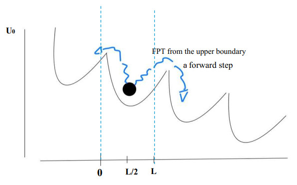
We propose two stochastic models for the interaction between the myosin head and the actin filament, the physio-chemical mechanism triggering muscle contraction and that is not yet completely understood. We make use of the fractional calculus approach with the purpose of constructing non-Markov processes for models with $ memory. $ A time-changed process and a fractionally integrated process are proposed for the two models. Each of these includes memory effects in a different way. We describe such features from a theoretical point of view and with simulations of sample paths. Mean functions and covariances are provided, considering constant and time-dependent tilting forces by which effects of external loads are included. The investigation of the dwell time of such phenomenon is carried out by means of density estimations of the first exit time (FET) of the processes from a strip; this mimics the times of the Steps of the myosin head during the sliding movement outside a potential well due to the interaction with actin. For the case of time-changed diffusion process, we specify an equation for the probability density function of the FET from a strip. The schemes of two simulation algorithms are provided and performed. Some numerical and simulation results are given and discussed.

References

[1]	M. O. Magnasco, G. Stolovitzky, Feynman's Ratchet and Pawl, J. Statist. Phys., 93 (1998), 615–632. https://doi.org/10.1023/B:JOSS.0000033245.43421.14 doi: 10.1023/B:JOSS.0000033245.43421.14
[2]	P. Reimann, Brownian motors: Noisy transport far from equilibrium, Phys. Rep., 361 (2002), 57–265. https://doi.org/10.1016/S0370-1573(01)00081-3 doi: 10.1016/S0370-1573(01)00081-3
[3]	H. Wang, G. Oster, Ratchets, power strokes, and molecular motors, Appl. Phys. A, 75 (2002), 315–323. https://doi.org/10.1007/s003390201340 doi: 10.1007/s003390201340
[4]	J. A. Spudich, How molecular motors work. Nature, 372 (1994), 515–518. https://doi.org/10.1038/372515a0 doi: 10.1038/372515a0
[5]	T. Masuda, Molecular dynamics simulation of a myosin subfragment-1 dockingwith an actin filament, BioSystems, 113 (2013), 144–148. https://doi.org/10.1016/j.biosystems.2013.06.001 doi: 10.1016/j.biosystems.2013.06.001
[6]	J. E. Molloy, J. E.Burns, J. Kendrick-Jones, R. T. Tregear, D. C. White, Movement and force produced by a single myosin head, Nature, 378 (1995), 209–212. https://doi.org/10.1038/378209a0 doi: 10.1038/378209a0
[7]	A. Buonocore, L. Caputo, Y. Ishii, E. Pirozzi, T. Yanagida, L. M. Ricciardi, On Myosin II dynamics in the presence of external loads, BioSystems, 81 (2005), 165–177. https://doi.org/10.1016/j.biosystems.2005.04.002 doi: 10.1016/j.biosystems.2005.04.002
[8]	S. Abdal, S. Hussain, I. Siddique, A. Ahmadian, M. Ferrara, On solution existence of MHD Casson nanofluid transportation across an extending cylinder through porous media and evaluation of priori bounds, Sci. Rep., 11 (2021), 7799. https://doi.org/10.1038/s41598-021-86953-1 doi: 10.1038/s41598-021-86953-1
[9]	K. Kitamura, M. Tokunaga, A. H. Iwane, T. Yanagida, A single myosin head moves along an actin filament with regular Steps of 5.3 nanometres, Nature, 397 (1999), 129–134. https://doi.org/10.1038/16403 doi: 10.1038/16403
[10]	G. D'Onofrio, E. Pirozzi, Two-boundary first exit time of Gauss-Markov processes for stochastic modeling of acto-myosin dynamics, J. Math. Biol., 74 (2017), 1511–1531. https://doi.org/10.1007/s00285-016-1061-x doi: 10.1007/s00285-016-1061-x
[11]	T. Masuda, A possible mechanism for determining the directionality of myosin molecular motors, Biosystems, 93 (2008), 172–180. https://doi.org/10.1016/j.biosystems.2008.03.009 doi: 10.1016/j.biosystems.2008.03.009
[12]	M. M. Meerschaert, A. Sikorskii, Stochastic Models for Fractional Calculus, in: series De Gruyter Studies in Mathematics, 43 (2012). https://doi.org/10.1515/9783110258165
[13]	D. Chalishajar, D. Geary, G. Cox, Review study of detection of diabetes models through delay differential equations, Appl. Math., 7 (2016), 1087–1102. http://dx.doi.org/10.4236/am.2016.710097 doi: 10.4236/am.2016.710097
[14]	D. Chalishajar, A. Stanford, Mathematical Analysis of Insulin-glucose feedback system of Detection of Diabetes, Int. J. Eng. Appl. Sci., 5 (2014), 36–58.
[15]	S. Jain, D. N. Chalishajar, Chikungunya Transmission of Mathematical Model Using the Fractional Derivative, Symmetry, 15 (2023), 952. https://doi.org/10.3390/sym15040952 doi: 10.3390/sym15040952
[16]	E. Pirozzi, Some fractional stochastic models for neuronal activity with different time-scales and correlated inputs, Fract. Fract., 8 (2024), 57. https://doi.org/10.3390/fractalfract8010057 doi: 10.3390/fractalfract8010057
[17]	S. Salahshour, A. Ahmadian, F. Ismail, D. Baleanu, N. Senu, A new fractional derivative for differential equation of fractional order under interval uncertainty, Adv. Mechan. Eng., 7 (2015). https://doi.org/10.1177/1687814015619138
[18]	N. Leonenko, M. M. Meerschaert, R. L. Schilling, A. Sikorskii, Correlation Structure of Time-Changed Lévy Processes, Commun. Appl. Indust. Math., (2014), e-483 https://doi.org/10.1685/journal.caim.483
[19]	N. Leonenko, E. Pirozzi, First passage times for some classes of fractional time-changed diffusions, Stochast. Anal. Appl., 40 (2021), 735-763. https://doi.org/10.1080/07362994.2021.1953386 doi: 10.1080/07362994.2021.1953386
[20]	M. Abundo, E. Pirozzi, Fractionally integrated Gauss-Markov processes and applications, Commun. Nonlinear Sci. Numer. Simul., 101 (2021), 105862. https://doi.org/10.1016/j.cnsns.2021.105862 doi: 10.1016/j.cnsns.2021.105862
[21]	D. Cyranoski, Swimming against the tide, Nature, 408 (2000), 764–766. https://doi.org/10.1038/35048748 doi: 10.1038/35048748
[22]	F. Oosawa, The loose coupling mechanism in molecular machines of living cells, Genes Cells, 5 (2000), 9–16. https://doi.org/10.1046/j.1365-2443.2000.00304.x doi: 10.1046/j.1365-2443.2000.00304.x
[23]	A. Buonocore, L. Caputo, E. Pirozzi, On a pulsating Brownian motor and its characterization, Math. Biosci., 207 (2007), 387–401. https://doi.org/10.1016/j.mbs.2006.11.013 doi: 10.1016/j.mbs.2006.11.013
[24]	A. Buonocore, L. Caputo, E. Pirozzi, L. M.Ricciardi, Simulation of Myosin II dynamics modeled by a pulsating ratchet with double-well potentials, in Lecture Notes in Computer Science, Computer Aided System Theory - EUROCAST (eds. R. Moreno-diaz, F. Pichler, A. Quesada-arencibia), Springer-Verlag, BERLIN, (2007), 154–162. https://doi.org/10.1007/978-3-540-75867-9_20
[25]	M. M. Meerschaert, P. Straka, Inverse stable subordinators, Math. Model. Natural Phenom., 8 (2013), 1–16. https://doi.org/10.1051/mmnp/20138201 doi: 10.1051/mmnp/20138201
[26]	G. Ascione, Y. Mishura, E. Pirozzi, Fractional deterministic and stochastic calculus, De Gruyter, 2024. https://doi.org/10.1515/9783110780017
[27]	E. Pirozzi, Colored noise and a stochastic fractional model for correlated inputs and adaptation in neuronal firing, Biol. Cybernet., 112 (2018), 25–39. https://doi.org/10.1007/s00422-017-0731-0 doi: 10.1007/s00422-017-0731-0
[28]	W. Teka, T. M. Marinov, F. Santamaria, Neuronal spike timing adaptation described with a fractional leaky Integrate-and-Fire model, PLoS Comput. Biol., 10 (2014). https://doi.org/10.1371/journal.pcbi.1003526
[29]	A. N. Kochubei, General fractional calculus, evolution equations, and renewal processes, Integr. Equ. Oper. Theory, 71 (2011), 583–600. https://doi.org/10.1007/s00020-011-1918-8
[30]	B. Toaldo, Convolution-Type Derivatives, Hitting-Times of Subordinators and Time-Changed C 0-semigroups, Potential Anal, 42 (2015), 115-140. https://doi.org/10.1007/s11118-014-9426-5 doi: 10.1007/s11118-014-9426-5
[31]	L. Arnold, Stochastic Differential Equations: Theory and Applications, Wiley-Interscience, (1974).
[32]	A. Buonocore, L. Caputo, E. Pirozzi, L. M. Ricciardi, The first passage time problem for Gauss-diffusion processes: Algorithmic approaches and applications to LIF neuronal model, Methodol. Comput. Appl. Probab., 13 (2011), 29–57. https://doi.org/10.1007/s11009-009-9132-8 doi: 10.1007/s11009-009-9132-8
[33]	E. Di Nardo, A. G. Nobile, E. Pirozzi, L. M. Ricciardi, A computational approach to first-passage-time problems for Gauss-Markov processes, Adv. Appl. Probab., 33 (2001), 453–482. https://doi.org/10.1017/S0001867800010892 doi: 10.1017/S0001867800010892
[34]	J. Bertoin, Lévy processes, Cambridge University Press, 121 (1996).
[35]	N. H. Bingham, Limit theorems for occupation times of Markov processes, Z. Wahrscheinlichkeitstheorie und Verw. Gebiete., 17 (1971), 1–22. https://doi.org/10.1007/BF00538470 doi: 10.1007/BF00538470
[36]	L. Bondesson, G. K. Kristiansen, F. W. Steutel, Infinite divisibility of random variables and their integer parts, Stat. Probab. Letters, 28 (1996), 271–278. https://doi.org/10.1016/0167-7152(95)00135-2 doi: 10.1016/0167-7152(95)00135-2
[37]	I. Gradshteyn, I. Ryzhik, Table of integrals, series, and products, Elsevier/Academic Press, Amsterdam, Seventh edition, (2007).
[38]	S. Bochner, Harmonic Analysis and the Theory of Probability, University of California Press, Berkeley, (1955). https://doi.org/10.1525/9780520345294
[39]	F. Mainardi, G. Pagnini, R. Gorenflo, Mellin transform and subordination laws in fractional diffusion processes, Fract. Calculus Appl. Anal., 6 (2003), 441–459.
[40]	H. Sato, Levy Processes and Infinitely Divisible Distributions, Cambridge University Press, (1999).
[41]	M. Hahn, J. Ryvkina, K. Kobayashi, S. Umarov, On time-changed Gaussian processes and their associated Fokker-Planck-Kolmogorov equations, Electron. Commun. Probab., 16 (2011), 150–164. https://doi.org/10.1214/ECP.v16-1620 doi: 10.1214/ECP.v16-1620
[42]	S. Umarov, Introduction to fractional and Pseudo-differential equations with singular symbols, Developments Math., 41 (2015). https://doi.org/10.1007/978-3-319-20771-1
[43]	F. Mainardi, On some properties of the Mittag-Leffler function $\mathbf{E_\alpha(-t^\alpha)}$, completely monotone for $\mathbf{t> 0}$ with $\mathbf{0 < \alpha < 1}$, Discrete Cont. Dynam. Syst. B, 19 (2014), 2267–2278. https://doi.org/10.3934/dcdsb.2014.19.2267 doi: 10.3934/dcdsb.2014.19.2267
[44]	A. G. Nobile, E. Pirozzi, L. M. Ricciardi, On the two-boundary first-passage time for a class of Markov processes, Sci. Math. Japon., 64 (2006), 421–442.
[45]	E. Pirozzi, Mittag–Leffler fractional stochastic integrals and processes with applications, Mathematics, 12 (2024), 3094. https://doi.org/10.3390/math12193094 doi: 10.3390/math12193094
[46]	P. T. Anh, T. S. Doan, P. T. Huong, A variation of constant formula for Caputo fractional stochastic differential equations, Stat. Probab. Letters, 145 (2019), 351–358. https://doi.org/10.1016/j.spl.2018.10.010 doi: 10.1016/j.spl.2018.10.010
[47]	M. G. Hahn, K. Kobayashi, S. Umarov, Fokker-Planck-Kolmogorov equations associated with time-changed fractional Brownian motion, Proceed. Am. Math. Soc., 139 (2011), 691-–705. https://doi.org/10.1090/S0002-9939-2010-10527-0 doi: 10.1090/S0002-9939-2010-10527-0
[48]	K. Kobayashi, Stochastic calculus for a time-changed Semimartingale and the associated stochastic differential equations, J. Theor. Probab., 24 (2011), 789-820. https://doi.org/10.1007/s10959-010-0320-9 doi: 10.1007/s10959-010-0320-9
[49]	T. S. Doan, P. Kloeden, P. Huong, H. T. Tuan, Asymptotic separation between solutions of Caputo fractional stochastic differential equations, Stoch. Anal. Appl., 36 (2018), 654-664. https://doi.org/10.1080/07362994.2018.1440243 doi: 10.1080/07362994.2018.1440243
[50]	K. Diethelm, The analysis of fractional differential equations, Lecture Notes in Mathematics, Springer-Verlag Berlin Heidelberg, (2010).
[51]	R. Garrappa, E. Kaslik, M. Popolizio, Evaluation of fractional integrals and derivatives of elementary functions: Overview and tutorial, Mathematics, 7 (2019), 407. https://doi.org/10.3390/math7050407 doi: 10.3390/math7050407
[52]	I. Podlubny, Fractional differential equations, An introduction to fractional derivatives, fractional differential equations, to methods of their solution and some of their applications, Academic Press, Inc., San Diego, CA, (2019).
[53]	G. Ascione, E. Pirozzi, Generalized fractional calculus for Gompertz-Type models, Mathematics, 9 (2021), 2140. https://doi.org/10.3390/math9172140 doi: 10.3390/math9172140
[54]	E. Jum, K. Kobayashi, A strong and weak approximation scheme for stochastic differential equations driven by a time-changed Brownian motion, Probab. Math. Statist., 36 (2016), 201-220.
[55]	S. X. Jin, K. Kobayashi, Strong approximation of stochastic differential equations driven by a time-changed Brownian motion with time-space-dependent coefficients, J. Math. Anal. Appl., 476 (2019), 619–636. https://doi.org/10.1016/j.jmaa.2019.04.001 doi: 10.1016/j.jmaa.2019.04.001
[56]	M. Magdziarz, A. Weron, K. Weron, Fractional Fokker-Planck dynamics: Stochastic representation and computer simulation, Phys. Rev. E, 75 (2007), 016708. https://doi.org/10.1103/PhysRevE.75.016708 doi: 10.1103/PhysRevE.75.016708

Reader Comments

Your name:*

Email:*
© 2025 the Author(s), licensee AIMS Press. This is an open access article distributed under the terms of the Creative Commons Attribution License (http://creativecommons.org/licenses/by/4.0)