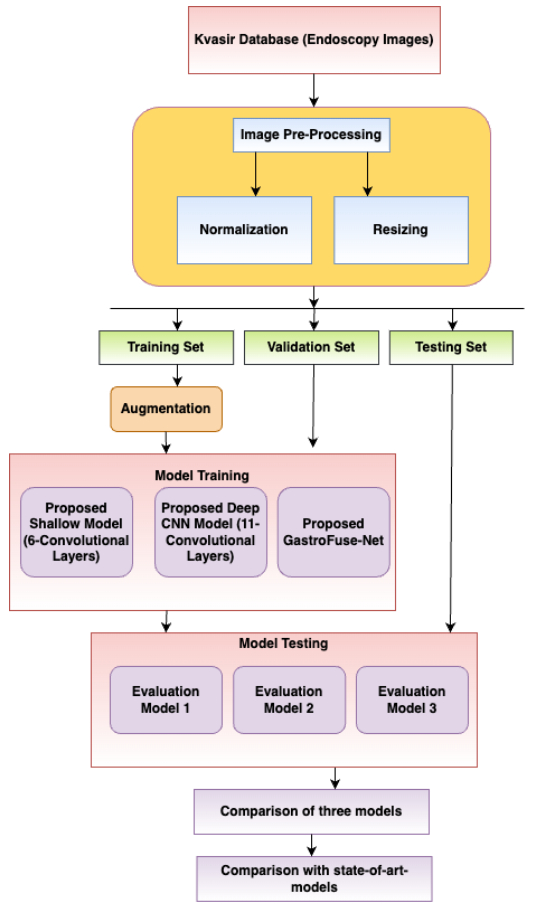
Convolutional Neural Networks (CNNs) have received substantial attention as a highly effective tool for analyzing medical images, notably in interpreting endoscopic images, due to their capacity to provide results equivalent to or exceeding those of medical specialists. This capability is particularly crucial in the realm of gastrointestinal disorders, where even experienced gastroenterologists find the automatic diagnosis of such conditions using endoscopic pictures to be a challenging endeavor. Currently, gastrointestinal findings in medical diagnosis are primarily determined by manual inspection by competent gastrointestinal endoscopists. This evaluation procedure is labor-intensive, time-consuming, and frequently results in high variability between laboratories. To address these challenges, we introduced a specialized CNN-based architecture called GastroFuse-Net, designed to recognize human gastrointestinal diseases from endoscopic images. GastroFuse-Net was developed by combining features extracted from two different CNN models with different numbers of layers, integrating shallow and deep representations to capture diverse aspects of the abnormalities. The Kvasir dataset was used to thoroughly test the proposed deep learning model. This dataset contained images that were classified according to structures (cecum, z-line, pylorus), diseases (ulcerative colitis, esophagitis, polyps), or surgical operations (dyed resection margins, dyed lifted polyps). The proposed model was evaluated using various measures, including specificity, recall, precision, F1-score, Mathew's Correlation Coefficient (MCC), and accuracy. The proposed model GastroFuse-Net exhibited exceptional performance, achieving a precision of 0.985, recall of 0.985, specificity of 0.984, F1-score of 0.997, MCC of 0.982, and an accuracy of 98.5%.
Citation: Sonam Aggarwal, Isha Gupta, Ashok Kumar, Sandeep Kautish, Abdulaziz S. Almazyad, Ali Wagdy Mohamed, Frank Werner, Mohammad Shokouhifar. GastroFuse-Net: an ensemble deep learning framework designed for gastrointestinal abnormality detection in endoscopic images[J]. Mathematical Biosciences and Engineering, 2024, 21(8): 6847-6869. doi: 10.3934/mbe.2024300
Convolutional Neural Networks (CNNs) have received substantial attention as a highly effective tool for analyzing medical images, notably in interpreting endoscopic images, due to their capacity to provide results equivalent to or exceeding those of medical specialists. This capability is particularly crucial in the realm of gastrointestinal disorders, where even experienced gastroenterologists find the automatic diagnosis of such conditions using endoscopic pictures to be a challenging endeavor. Currently, gastrointestinal findings in medical diagnosis are primarily determined by manual inspection by competent gastrointestinal endoscopists. This evaluation procedure is labor-intensive, time-consuming, and frequently results in high variability between laboratories. To address these challenges, we introduced a specialized CNN-based architecture called GastroFuse-Net, designed to recognize human gastrointestinal diseases from endoscopic images. GastroFuse-Net was developed by combining features extracted from two different CNN models with different numbers of layers, integrating shallow and deep representations to capture diverse aspects of the abnormalities. The Kvasir dataset was used to thoroughly test the proposed deep learning model. This dataset contained images that were classified according to structures (cecum, z-line, pylorus), diseases (ulcerative colitis, esophagitis, polyps), or surgical operations (dyed resection margins, dyed lifted polyps). The proposed model was evaluated using various measures, including specificity, recall, precision, F1-score, Mathew's Correlation Coefficient (MCC), and accuracy. The proposed model GastroFuse-Net exhibited exceptional performance, achieving a precision of 0.985, recall of 0.985, specificity of 0.984, F1-score of 0.997, MCC of 0.982, and an accuracy of 98.5%.

| [1] |
H. Brenner, M. Kloor, C. P. Pox, Colorectal cancer, Lancet, 383, (2014), 1490–1502. https://doi.org/10.1016/S0140-6736(13)61649-9 doi: 10.1016/S0140-6736(13)61649-9

|
| [2] |
M. F. Kaminski, J. Regula, E. Kraszewska, M. Polkowski, U. Wojciechowska, J. Didkowska, et al., Quality indicators for colonoscopy and the risk of interval cancer, N. Engl. J. Med., 362 (2010), 1795–1803. https://doi.org/10.1056/nejmoa0907667 doi: 10.1056/nejmoa0907667
|
| [3] |
T. Takahashi, Y. Saikawa, Y. Kitagawa, Gastric cancer: current status of diagnosis and treatment, Cancers (Basel), 5 (2013), 48–63. https://doi.org/10.3390/cancers5010048 doi: 10.3390/cancers5010048
|
| [4] |
T. Yada, C. Yokoi, N. Uemura, The current state of diagnosis and treatment for early gastric cancer, Diagn. Ther. Endosc., 2013 (2013), 24132. https://doi.org/10.1155/2013/241320 doi: 10.1155/2013/241320
|
| [5] |
A. Shokouhifar, M. Shokouhifar, M. Sabbaghian, H. Soltanian-Zadeh, Swarm intelligence empowered three-stage ensemble deep learning for arm volume measurement in patients with lymphedema, Biomed. Signal Process. Control, 85 (2023), 105027. https://doi.org/10.1016/j.bspc.2023.105027 doi: 10.1016/j.bspc.2023.105027
|
| [6] |
E. J. Topol, High-performance medicine: the convergence of human and artificial intelligence, Nat. Med., 25 (2019), 44−56. https://doi.org/10.1038/s41591-018-0300-7 doi: 10.1038/s41591-018-0300-7
|
| [7] |
N. Sharma, S. Gupta, A. Rajab, M. A. Elmagzoub, K. Rajab, A. Shaikh, Semantic Segmentation of Gastrointestinal Tract in MRI Scans Using PSPNet Model With ResNet34 Feature Encoding Network, IEEE Access, 11 (2023), 132532−132543. https://doi.org/10.1109/ACCESS.2023.3336862 doi: 10.1109/ACCESS.2023.3336862
|
| [8] |
N. Sharma, S. Gupta, D. Koundal, S. Alyami, H. Alshahrani, Y. Asiri, et al., U-Net model with transfer learning model as a backbone for segmentation of gastrointestinal tract, Bioengineering (Basel), 10 (2023), 119. https://doi.org/10.3390/bioengineering10010119 doi: 10.3390/bioengineering10010119
|
| [9] |
J. Yang, M. Shokouhifar, L. Yee, A. A. Khan, M. Awais, Z. Mousavi, DT2F-TLNet: A novel text-independent writer identification and verification model using a combination of deep type-2 fuzzy architecture and Transfer Learning networks based on handwriting data, Expert Syst. Appl., 242 (2024), 122704. https://doi.org/10.1016/j.eswa.2023.122704 doi: 10.1016/j.eswa.2023.122704
|
| [10] |
A. Sharma, R. Kumar, P. Garg, Deep learning-based prediction model for diagnosing gastrointestinal diseases using endoscopy images, Int. J. Med. Inform., 177 (2023), 105142. https://doi.org/10.1016/j.ijmedinf.2023.105142 doi: 10.1016/j.ijmedinf.2023.105142
|
| [11] |
V. Raut, R. Gunjan, V. V. Shete, U. D. Eknath, Gastrointestinal tract disease segmentation and classification in wireless capsule endoscopy using intelligent deep learning model, Comput. Method. Biomec., 11 (2023), 606−622. https://doi.org/10.1080/21681163.2022.2099298 doi: 10.1080/21681163.2022.2099298
|
| [12] |
K. Zhang, Y. Zhang, Y. Ding, M. Wang, P. Bai, X. Wang, et al., Anatomical sites identification in both ordinary and capsule gastroduodenoscopy via deep learning, Biomed. Signal Proces., 90 (2024), 105911. https://doi.org/10.1016/j.bspc.2023.105911 doi: 10.1016/j.bspc.2023.105911
|
| [13] |
Y. Mori, S. E. Kudo, M. Misawa, Y. Saito, H. Ikematsu, K. Hotta, et al., Real-time use of artificial intelligence in identification of diminutive polyps during colonoscopy: A prospective study, Ann. Intern. Med., 169 (2018), 357–366. https://doi.org/10.7326/M18-0249 doi: 10.7326/M18-0249
|
| [14] |
C. M. Hsu, C. C. Hsu, Z. M. Hsu, T. H. Chen, T. Kuo, Intraprocedure Artificial Intelligence Alert System for Colonoscopy Examination, Sensors, 23 (2023), 1211. https://doi.org/10.3390/s23031211 doi: 10.3390/s23031211
|
| [15] |
E. Young, L. Edwards, R. Singh, The Role of Artificial Intelligence in Colorectal Cancer Screening: Lesion Detection and Lesion Characterization, Cancers, 15 (2023), 5126. https://doi.org/10.3390/cancers15215126 doi: 10.3390/cancers15215126
|
| [16] |
D. K. Iakovidis, A. Koulaouzidis, Software for enhanced video capsule endoscopy: challenges for essential progress, Nat. Rev. Gastroenterol. Hepatol., 12 (2015), 172–186. https://doi.org/10.1038/nrgastro.2015.13 doi: 10.1038/nrgastro.2015.13
|
| [17] |
S. A. Karkanis, D. K. Iakovidis, D. E. Maroulis, D. A. Karras, M. Tzivras, Computer-aided tumor detection in endoscopic video using color wavelet features, IEEE Trans. Inf. Technol. Biomed., 7, (2003), 141–152. https://doi.org/10.1109/TITB.2003.813794 doi: 10.1109/TITB.2003.813794
|
| [18] |
M. Liedlgruber, A. Uhl, Computer-aided decision support systems for endoscopy in the gastrointestinal tract: a review, IEEE Rev. Biomed. Eng., 4 (2011), 73–88. https://doi.org/10.1109/RBME.2011.2175445 doi: 10.1109/RBME.2011.2175445
|
| [19] | Y. Mori, K. Mori, Endoscopy: Computer-aided diagnostic system based on deep learning which supports endoscopists' decision-making on the treatment of colorectal polyps, In: Hashizume, M. (eds) Multidisciplinary Computational Anatomy. Springer, Singapore, 2022,337–342. https://doi.org/10.1007/978-981-16-4325-5_45 |
| [20] | K. Pogorelov, K. R. Randel, C. Griwodz, S. L. Eskeland, T. de Lange, D. Johansen, et al., Kvasir: A multi-class image dataset for computer aided gastrointestinal disease detection, in Proceedings of the 8th ACM multimedia systems conference, MMSys, (2017), 164–169. https://doi.org/10.1145/3083187.3083212 |
| [21] |
U. K. Lilhore, M. Poongodi, A. Kaur, S. Simaiya, A. D. Algarni, H. Elmannai, et al., Hybrid model for detection of cervical cancer using causal analysis and machine learning techniques, Comput. Math. Methods Med., 2022 (2022), 4688327. https://doi.org/10.1155/2022/4688327 doi: 10.1155/2022/4688327
|
| [22] |
W. S. Liew, T. B. Tang, C. H. Lin, C. K. Lu, Automatic colonic polyp detection using integration of modified deep residual convolutional neural network and ensemble learning approaches, Comput. Meth. Prog. Biomed., 206 (2021), 106114. https://doi.org/10.1016/j.cmpb.2021.106114 doi: 10.1016/j.cmpb.2021.106114
|
| [23] |
C. M. Lo, Y. W. Yang, J. K. Lin, T. C. Lin, W. S. Chen, S. H. Yang, et al., Modeling the survival of colorectal cancer patients based on colonoscopic features in a feature ensemble vision transformer, Comput. Med. Imag. Grap., 107 (2023), 102242. https://doi.org/10.1016/j.compmedimag.2023.102242 doi: 10.1016/j.compmedimag.2023.102242
|
| [24] |
H. Ali, M. Sharif, M. Yasmin, M. H. Rehmani, F. Riaz, A survey of feature extraction and fusion of deep learning for detection of abnormalities in video endoscopy of gastrointestinal tract, Artif. Intell. Rev., 53 (2020), 2635–2707. https://doi.org/10.1007/s10462-019-09743-2 doi: 10.1007/s10462-019-09743-2
|
| [25] |
D. Jha, S. Ali, S. Hicks, V. Thambawita, H. Borgli, P. Smedsrud, et al., A comprehensive analysis of classification methods in gastrointestinal endoscopy imaging, Med. Image Anal., 70 (2021), 102007. https://doi.org/10.1016/j.media.2021.102007 doi: 10.1016/j.media.2021.102007
|
| [26] | S. S. A. Naqvi, S. Nadeem, M. Zaid, M. A. Tahir, Ensemble of texture features for finding abnormalities in the gastrointestinal tract, in MediaEval Benchmarking Initiative for Multimedia Evaluation, 2017. Available from: https://api.semanticscholar.org/CorpusID:6396180 |
| [27] |
M. Billah, S. Waheed, Gastrointestinal polyp detection in endoscopic images using an improved feature extraction method, Biomed. Eng. Lett., 8 (2018), 69–75. https://doi.org/10.1007/s13534-017-0048-x doi: 10.1007/s13534-017-0048-x
|
| [28] |
A. Rosenfeld, D. G. Graham, S. Jevons, J. Ariza, D. Hagan, A. Wilson, et al., Development and validation of a risk prediction model to diagnose Barrett's oesophagus (MARK-BE): a case-control machine learning approach, Lancet Digit. Health, 2 (2020), E37–E48. https://doi.org/10.1016/S2589-7500(19)30216-X doi: 10.1016/S2589-7500(19)30216-X
|
| [29] |
K. Kundu, S. A. Fattah, K. A. Wahid, Multiple linear discriminant models for extracting salient characteristic patterns in capsule endoscopy images for multi-disease detection, IEEE J. Transl. Eng. Health Med., 8 (2020), 3300111. https://doi.org/10.1109/JTEHM.2020.2964666 doi: 10.1109/JTEHM.2020.2964666
|
| [30] | T. Agrawal, R. Gupta, S. Sahu, C. E. Wilson, SCL-UMD at the medico task-mediaeval 2017: Transfer learning-based classification of medical images, MediaEva, 17 (2017), 13–15. |
| [31] | S. Petscharnig, K. Schoffmann, M. Lux, An inception-like CNN architecture for GI disease and anatomical landmark classification, MediaEva, 17 (2017), 13–15. |
| [32] | H. Gammulle, S. Denman, S. Sridharan,C. Fookes, Two-stream deep feature modelling for automated video endoscopy data analysis, In Medical Image Computing and Computer Assisted Intervention – MICCAI 2020: 23rd International Conference, Lima, Peru, October 4-8, 2020, Proceedings, Part Ⅲ 23. Springer International Publishing, 2020,742–751. https://doi.org/10.1007/978-3-030-59716-0_71 |
| [33] |
T. Cogan, M. Cogan, L. Tamil, MAPGI: Accurate identification of anatomical landmarks and diseased tissue in gastrointestinal tract using deep learning, Comput. Biol. Med., 111 (2019), 103351. https://doi.org/10.1016/j.compbiomed.2019.103351 doi: 10.1016/j.compbiomed.2019.103351
|
| [34] |
S. Jain, A. Seal, A. Ojha, A. Yazidi, J. Bures, I. Tacheci, et al., A deep CNN model for anomaly detection and localization in wireless capsule endoscopy images, Comput. Biol. Med., 137 (2021), 104789. https://doi.org/10.1016/j.media.2021.102007 doi: 10.1016/j.media.2021.102007
|
| [35] |
S. Mohapatra, G. Kumar Pati, M. Mishra, T. Swarnkar, Gastrointestinal abnormality detection and classification using empirical wavelet transform and deep convolutional neural network from endoscopic images, Ain Shams Eng. J., 14 (2023), 101942. https://doi.org/10.1016/j.asej.2022.101942 doi: 10.1016/j.asej.2022.101942
|
| [36] |
T. Abraham, J. V. Muralidhar, A. Sathyarajasekaran, K. Ilakiyaselvan, A Deep-Learning Approach for Identifying and Classifying Digestive Diseases, Symmetry, 15 (2023), 379. https://doi.org/10.3390/sym15020379 doi: 10.3390/sym15020379
|
| [37] | C. Gamage, I. Wijesinghe, C. Chitraranjan, I. Perera, GI-Net: Anomalies classification in gastrointestinal tract through endoscopic imagery with deep learning, in 2019 Moratuwa Engineering Research Conference (MERCon), 2019. https://doi.org/10.1109/MERCon.2019.8818929 |
| [38] |
J. Yogapriya, V. Chandran, M. G. Sumithra, P. Anitha, P. Jenopaul, C. Suresh Gnana Dhas, Gastrointestinal tract disease classification from wireless endoscopy images using pretrained deep learning model, Comput. Math. Methods Med., 2021 (2021), 5940433. https://doi.org/10.1155/2021/5940433. doi: 10.1155/2021/5940433
|
| [39] |
M. Khan, K. Muhammad, S. H. Wang, S. Alsubai, A. Binbusayyis, A. Alqahtani, et al., Gastrointestinal diseases recognition: a framework of deep neural network and improved moth-crow optimization with DCCA fusion, Hum-Cent. Comput. Info. Sci., 12 (2022), 1–12. https://doi.org/10.22967/HCIS.2022.12.025 doi: 10.22967/HCIS.2022.12.025
|


Figures(11) / Tables(6)

Sonam Aggarwal, Isha Gupta, Ashok Kumar, Sandeep Kautish, Abdulaziz S. Almazyad, Ali Wagdy Mohamed, Frank Werner, Mohammad Shokouhifar. GastroFuse-Net: an ensemble deep learning framework designed for gastrointestinal abnormality detection in endoscopic images[J]. Mathematical Biosciences and Engineering, 2024, 21(8): 6847-6869. doi: 10.3934/mbe.2024300


 DownLoad: