Figure 1.
Interval type-2 fuzzy relation unknown.


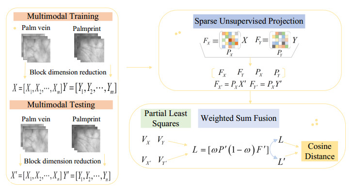
Biometric authentication prevents losses from identity misuse in the artificial intelligence (AI) era. The fusion method integrates palmprint and palm vein features, leveraging their stability and security and enhances counterfeiting prevention and overall system efficiency through multimodal correlations. However, most of the existing multi-modal palmprint and palm vein feature extraction methods extract only feature information independently from different modalities, ignoring the importance of the correlation between different modal samples in the class to the improvement of recognition performance. In this study, we addressed the aforementioned issues by proposing a feature-level joint learning fusion approach for palmprint and palm vein recognition based on modal correlations. The method employs a sparse unsupervised projection algorithm with a "purification matrix" constraint to enhance consistency in intra-modal features. This minimizes data reconstruction errors, eliminating noise and extracting compact, and discriminative representations. Subsequently, the partial least squares algorithm extracts high grayscale variance and category correlation subspaces from each modality. A weighted sum is then utilized to dynamically optimize the contribution of each modality for effective classification recognition. Experimental evaluations conducted for five multimodal databases, composed of six unimodal databases including the Chinese Academy of Sciences multispectral palmprint and palm vein databases, yielded equal error rates (EER) of 0.0173%, 0.0192%, 0.0059%, 0.0010%, and 0.0008%. Compared to some classical methods for palmprint and palm vein fusion recognition, the algorithm significantly improves recognition performance. The algorithm is suitable for identity recognition in scenarios with high security requirements and holds practical value.
Citation: Wei Wu, Yuan Zhang, Yunpeng Li, Chuanyang Li. Fusion recognition of palmprint and palm vein based on modal correlation[J]. Mathematical Biosciences and Engineering, 2024, 21(2): 3129-3145. doi: 10.3934/mbe.2024139
| [1] | Ruohan Cao, Jin Su, Jinqian Feng, Qin Guo . PhyICNet: Physics-informed interactive learning convolutional recurrent network for spatiotemporal dynamics. Electronic Research Archive, 2024, 32(12): 6641-6659. doi: 10.3934/era.2024310 |
| [2] | Ishtiaq Ali . Advanced machine learning technique for solving elliptic partial differential equations using Legendre spectral neural networks. Electronic Research Archive, 2025, 33(2): 826-848. doi: 10.3934/era.2025037 |
| [3] | Li Tian, Ziqiang Wang, Junying Cao . A high-order numerical scheme for right Caputo fractional differential equations with uniform accuracy. Electronic Research Archive, 2022, 30(10): 3825-3854. doi: 10.3934/era.2022195 |
| [4] | Jinjun Yong, Xianbing Luo, Shuyu Sun . Deep multi-input and multi-output operator networks method for optimal control of PDEs. Electronic Research Archive, 2024, 32(7): 4291-4320. doi: 10.3934/era.2024193 |
| [5] | Dewang Li, Meilan Qiu, Jianming Jiang, Shuiping Yang . The application of an optimized fractional order accumulated grey model with variable parameters in the total energy consumption of Jiangsu Province and the consumption level of Chinese residents. Electronic Research Archive, 2022, 30(3): 798-812. doi: 10.3934/era.2022042 |
| [6] | Yiyuan Qian, Kai Zhang, Jingzhi Li, Xiaoshen Wang . Adaptive neural network surrogate model for solving the implied volatility of time-dependent American option via Bayesian inference. Electronic Research Archive, 2022, 30(6): 2335-2355. doi: 10.3934/era.2022119 |
| [7] | Simon Eberle, Arnulf Jentzen, Adrian Riekert, Georg S. Weiss . Existence, uniqueness, and convergence rates for gradient flows in the training of artificial neural networks with ReLU activation. Electronic Research Archive, 2023, 31(5): 2519-2554. doi: 10.3934/era.2023128 |
| [8] | Jun Guo, Yanchao Shi, Weihua Luo, Yanzhao Cheng, Shengye Wang . Exponential projective synchronization analysis for quaternion-valued memristor-based neural networks with time delays. Electronic Research Archive, 2023, 31(9): 5609-5631. doi: 10.3934/era.2023285 |
| [9] | Huanhuan Li, Lei Kang, Meng Li, Xianbing Luo, Shuwen Xiang . Hamiltonian conserved Crank-Nicolson schemes for a semi-linear wave equation based on the exponential scalar auxiliary variables approach. Electronic Research Archive, 2024, 32(7): 4433-4453. doi: 10.3934/era.2024200 |
| [10] | Jye Ying Sia, Yong Kheng Goh, How Hui Liew, Yun Fah Chang . Constructing hidden differential equations using a data-driven approach with the alternating direction method of multipliers (ADMM). Electronic Research Archive, 2025, 33(2): 890-906. doi: 10.3934/era.2025040 |
Biometric authentication prevents losses from identity misuse in the artificial intelligence (AI) era. The fusion method integrates palmprint and palm vein features, leveraging their stability and security and enhances counterfeiting prevention and overall system efficiency through multimodal correlations. However, most of the existing multi-modal palmprint and palm vein feature extraction methods extract only feature information independently from different modalities, ignoring the importance of the correlation between different modal samples in the class to the improvement of recognition performance. In this study, we addressed the aforementioned issues by proposing a feature-level joint learning fusion approach for palmprint and palm vein recognition based on modal correlations. The method employs a sparse unsupervised projection algorithm with a "purification matrix" constraint to enhance consistency in intra-modal features. This minimizes data reconstruction errors, eliminating noise and extracting compact, and discriminative representations. Subsequently, the partial least squares algorithm extracts high grayscale variance and category correlation subspaces from each modality. A weighted sum is then utilized to dynamically optimize the contribution of each modality for effective classification recognition. Experimental evaluations conducted for five multimodal databases, composed of six unimodal databases including the Chinese Academy of Sciences multispectral palmprint and palm vein databases, yielded equal error rates (EER) of 0.0173%, 0.0192%, 0.0059%, 0.0010%, and 0.0008%. Compared to some classical methods for palmprint and palm vein fusion recognition, the algorithm significantly improves recognition performance. The algorithm is suitable for identity recognition in scenarios with high security requirements and holds practical value.
The concept of type-2 fuzzy sets (T2 FSs) was first proposed by Zadeh [1] and a detailed introduction was given in [2]. T2 FSs are an extension of the type-1 fuzzy set (T1 FS) and further considers the fuzziness of the fuzzy set. Since the definition of T2 FSs was proposed, most scholars have mainly studied the operations and properties of T2 FSs [3,4]. Until the 1990s, Prof. Mendel redefined T2 FSs and proposed the type-2 fuzzy logic system (T2 FLS) [5,6].
As an extension of T1 FSs, T2 FSs overcome the limitations of T1 FSs in dealing with the uncertainties of actual objects. However the definition of T2 FSs is complicated, and the corresponding graph must be a spatial graph. Due to the complexity of the expression of T2 FSs, Mendel introduces the definition of interval T2 FSs (IT2 FSs) as a special case of T2 FSs. The secondary membership grade of IT2 FSs is constant one, which is more simpler than T2 FSs. In general, IT2 fuzzy logic system (IT2 FLS) are used in most theories and applications [7,8].
In the field of fuzzy control, solving fuzzy relation equations (FREs) plays an important role in the design of fuzzy controller and fuzzy logic reasoning. Most algorithms for solving FREs can obtain some specific solutions, such as the minimum or maximum solution [9], or can describe the solution theoretically [10]. In the existing methods, most of them are used for solving type-1 fuzzy relation equations (T1 FREs), while few methods are used for solving interval type-2 fuzzy relation equations (IT2 FREs). The main work of this paper is to propose a new method to obtain the entire solution set of IT2 FREs.
On the other hand, Prof. Cheng proposed a new matrix product-semi-tensor product (STP) of matrices, which is the generalization of the conventional matrix product and retains almost all the main properties of the conventional matrix product. As a novel mathematical technique for handling logical operations, STP has been successfully applied to logical systems [11,12,13,14] and, based on this, a new algorithm for solving FREs has been devised. For example, in T1 FREs, the STP is used to solve fuzzy relation equalities and fuzzy relation inequalities [15,16,17,18]. In type-2 fuzzy relational equations (T2 FREs), only some simple algorithms have been proposed to study the solution of type-2 single-valued fuzzy relation equations and type-2 symmetry-valued fuzzy relation equations [19,20]. However, the ordinary STP cannot be used directly to solve IT2 FREs. Therefore, we extend the STP to interval matrices and propose the STP of interval matrices, then discuss the solutions of IT2 FREs.
In the rest of this paper, section two introduces the basic concepts of the STP of interval matrices. Section three mainly gives the relevant definitions of interval-valued logic and gives its matrix representation. Section four discusses the solvability of IT2 FREs and designs an algorithm to solve IT2 FREs. Section five explains the viability of the proposed algorithm with a numerical example. Section six gives a brief summary of the paper.
First, in order to express conveniently, we introduce some notations used throughout the paper.
●
| I[0,1]:={[α_,¯α]|0≤α_≤¯α≤1}, |
where α_,¯α∈R. If α=[α_,α_](or α=[¯α,¯α]), this is a point interval and α degenerates into a real number.
●
| I([0,1]m):={[A_,¯A]|A_≤¯A}. |
A_=(α_i)m and ¯A=(¯αi)m are two m-dimensional vectors and [a_i,¯ai]∈I[0,1], i=1⋯m.
●
| I([0,1]m×n):={[A_,¯A]|A_≤¯A}. |
A_=(α_ij)m×n and ¯A=(¯αij)m×n are two m×n dimensional matrices and [α_ij,¯αij]∈I[0,1], i=1⋯m, j=1⋯n.
● δir : the ith column of unit matrix In.
● [δir,δjr] : a bounded closed interval, where δin represents its lower bound and δjn represents its upper bound, abbreviated as δr[i,j].
● Coli(M): the ith column of interval matrix M.
● Rowj(M): the jth row of interval matrix M.
Next, we define ∧,∨ and ¬ in I[0,1].
Definition 2.1. [21] (1) Let
| α=[α_,¯α], β=[β_,¯β]∈I[0,1], |
then,
| α∨β=[max(α_,β_),max(¯α,¯β)], | (2.1) |
| α∧β=[min(α_,β_),min(¯α,¯β)]. | (2.2) |
(2) Let
| A=[a_ij,¯aij]∈I([0,1]m×n), |
| B=[b_jk,¯bjk]∈I([0,1]n×p), |
then their max-min composition operation is defined as
| A∘B=C=[c_ik,¯cik]∈I([0,1]m×p), | (2.3) |
where
| [c_ik,¯cik]=([a_i1,¯ai1]∧[b_1k,¯b1k])∨([a_i2,¯ai2]∧[b_2k,¯b2k]) ∨⋯∨([a_in,¯ain]∧[b_nk,¯bnk]), |
where i=1,⋯,m, j=1,⋯,k.
Definition 2.2. [22] Let
| A=[a_ij,¯aij], |
| B=[b_ij,¯bij]∈I([0,1]m×n), |
then the partial order ≥,≤ and = are defined as
(1) If a_ij≥b_ij,¯aij≥¯bij, we say A≥B.
(2) If a_ij≤b_ij,¯aij≤¯bij, we say A≤B.
(3) If a_ij=b_ij,¯aij=¯bij, we say A=B.
Property 2.1. [15] Let
| A=[a_ij,¯aij], B=[b_ij,¯bij]∈I([0,1]m×n), |
| C=[c_jk,¯cjk], D=[d_jk,¯djk]∈I([0,1]n×p). |
Assume A≤B and C≤D, then
| A∘C≤B∘D. |
Definition 2.3. [22] (1) Let
| α=[α_,¯α], β=[β_,¯β]∈I[0,1], |
then the four operations of intervals α and β are as follows.
1) Addition operation
| α+β=[α_,¯α]+[β_,¯β]=[α_+β_,¯α+¯β]. | (2.4) |
2) Subtraction operation
| α−β=[α_,¯α]−[β_,¯β]=[α_−¯β,¯α−β_]. | (2.5) |
3) Multiplication operation
| α×β=[α_,¯α]×[β_,¯β]=[α_β_,¯α¯β]. | (2.6) |
4) Division operation
| α/β=[α_,¯α]/[β_,¯β]=[min(α_/β_,α_/¯β,¯α/β_,¯α/¯β),max(α_/β_,α_/¯β,¯α/β_,¯α/¯β)]. | (2.7) |
Note that 0∉β=[β_,¯β].
(2) If
| α=[α_,¯α]∈I[0,1], |
| A=[a_ij,¯aij]m×n∈I([0,1]m×n), |
then the product of interval α and interval matrix A is
| α×A:=([α_,¯α]×[a_ij,¯aij])m×n. | (2.8) |
(3) If
| A=[a_ij,¯aij]m×n∈I([0,1]m×n), |
| B=[b_jk,¯bjk]n×p∈I([0,1]n×p), |
then the product of interval matrices A and B is
| A×B=C=[c_ik,¯cik]n×p=[[c_11,¯c11]⋯[c_1p,¯c1p]⋮⋱⋮[c_n1,¯cn1]⋯[c_np,¯cnp]], | (2.9) |
where
| [c_ik,¯cik]=m∑j=1[a_ij,¯aij]×[b_jk,¯bjk]=[a_i1,¯ai1]×[b_1k,¯b1k]+[a_i2,¯ai2]×[b_2k,¯b2k]+⋯+[a_im,¯aim]×[b_mk,¯bmk]. |
Based on Definition 2.3, we give the relevant definition of the STP of interval matrices.
Definition 2.4. (1) If
| A=[a_ij,¯aij]m×n∈I([0,1]m×n), |
| B=[b_kl,¯bkl]p×q∈I([0,1]p×q), |
then the kronecker product of interval matrices A and B is
| A⊗B=[a11×B⋯a1n×B⋮⋱⋮am1×B⋯amn×B]. | (2.10) |
(2) If
| A=[a_ij,¯aij]m×n∈I([0,1]m×n), |
| B=[b_kl,¯bkl]p×q∈I([0,1]p×q), |
then the STP of interval matrices A and B is
| A⋉B=(A⊗Itn)×(B⊗Itp), | (2.11) |
where t=lcm(n,p) is the least common multiple of n and p.
(3) If
| A=[a_ij,¯aij]m×n∈I([0,1]m×n), |
| B=[b_kl,¯bkl]p×n∈I([0,1]p×n), |
then the khatri-rao product of interval matrices A and B is
| A∗B=[Col1(A)⋉Col1(B) Col2(A)⋉Col2(B)⋯Coln(A)⋉Coln(B)]. | (2.12) |
Remark 2.1. In Definition 2.4, if n=p, then the STP of interval matrices degenerates to the ordinary interval matrix multiplication. Therefore, the STP of interval matrices is a generalization of interval matrices multiplication. In the context, the STP of interval matrices is ⋉, which is omitted by default.
Example 2.1. Given the interval matrices A and B,
| A=[[0.2,0.4][0.4,0.5][0.6,1.0][0.8,0.9]], B=[[0,1][0.2,0.3][0.4,0.6][0.6,0.7][0.8,0.9][1,1][0.7,0.9][0.3,0.4]]. |
The kronecker product of the interval matrix A and the unit interval matrix I2 is
| A⊗I2=[[0.2,0.4][0,0][0.4,0.5][0,0][0,0][0.2,0.4][0,0][0.4,0.5][0.6,1.0][0,0][0.8,0.9][0,0][0,0][0.6,1.0][0,0][0.8,0.9]]. |
The STP of interval matrices A and B is
| A⋉BΔ=(A⊗I2)×B=[[0.16,0.70][0.28,0.47][0.32,1.54][0.60,0.93][0.44,0.81][0.32,0.60][1.04,1.71][0.84,1.36]]. |
The khatri-rao product of interval matrices A and B is
| A∗B=[Col1(A)×Col1(B)Col2(A)×Col2(B)]=[[0.00,0.40][0.04,0.12][0.08,0.24][0.12,0.28][0.32,0.45][0.40,0.50][0.28,0.45][0.12,0.20][0.00,1.00][0.12,0.30][0.24,0.60][0.36,0.70][0.64,0.81][0.80,0.90][0.56,0.81][0.24,0.32]]T. |
According to the definition of STP of interval matrices, we can get the following properties.
Property 2.2. (1) Let A,B∈I([0,1]m×n),C∈I([0,1]p×q), then
| (A+B)⋉C=A⋉C+B⋉C,C⋉(A+B)=C⋉A+C⋉B. | (2.13) |
(2) Let A∈I([0,1]m×n),B∈I([0,1]p×q) and C∈I([0,1]r×s), then
| (A⋉B)⋉C=A⋉(B⋉C). | (2.14) |
(3) Let A∈I([0,1]m×n), C∈I([0,1]s) and R∈I([0,1]s) are column and row interval vectors, respectively, then
| C⋉A=(Is⊗A)⋉C,R⋉A=(A⊗Is)⋉R. | (2.15) |
Let the interval type-2 fuzzy relation ˜R∈F(V×W), where the domain V={v1,v2,⋯,vn} and W={w1,w2,⋯,wp}, then the matrix form of interval type-2 fuzzy relation ˜R can be defined as
| M˜R=[f˜R(v1,w1)μ˜R(v1,w1)⋯f˜R(v1,wp)μ˜R(v1,wp)⋮⋱⋮f˜R(vn,w1)μ˜R(vn,w1)⋯f˜R(vn,wp)μ˜R(vn,wp)]. | (2.16) |
μ˜R(vi,wk) and f˜R(vi,wk) represent the primary membership grade and secondary membership grade of IT2 FSs, respectively. For primary membership grade, it is composed of upper membership grade and lower membership grade; that is,
| μ˜R(vi,wk)=[μ_˜R(vi,wk),¯μ˜R(vi,wk)]. |
The secondary membership grade of IT2 FSs equals one; that is, f˜R(vi,wk)=1, then the matrix form of interval type-2 fuzzy relation ˜R can be further described as
| M˜R=[1[μ_˜R(v1,w1),¯μ˜R(v1,w1)]⋯1[μ_˜R(v1,ws),¯μ˜R(v1,wp)]⋮⋱⋮1[μ_˜R(vn,w1),¯μ˜R(vn,w1)]⋯1[μ_˜R(vn,ws),¯μ˜R(vn,wp)]]. | (2.17) |
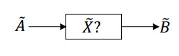
Two common types of FREs exist in practical application [20]. One type is that the fuzzy relation is unknown, which is commonly used for designing fuzzy controllers. The other type is that the fuzzy input is unknown, which is commonly used for diagnosing diseases based on the symptom similarity. In terms of the aforementioned situations, it can be assumed that there are similar two types of IT2 FREs, as shown in Figures 1 and 2.

Type 1: assume ˜A∈F(U×V),˜B∈F(U×W). We seek an interval type-2 fuzzy relation ˜X∈F(V×W) such that it satisfies
| ˜A∘˜X=˜B. | (2.18) |
Type 2: assume ˜R∈F(V×W),˜B∈F(U×W). We seek an interval type-2 fuzzy input ˜X∈F(U×V) such that it satisfies
| ˜X∘˜R=˜B. | (2.19) |
Remark 2.2. Take a transpose of both sides of (2.19) to get ˜RT∘˜XT=˜BT. (2.19) is equivalent to (2.18), so we only need to consider the solvability of (2.18).
Definition 3.1. (1)
| If={[α_,¯α]|0≤α_≤¯α≤1} |
is called the domain of interval-valued fuzzy logic, and the interval-valued fuzzy logic variable is P∈If. When α=[0,0] (orα=[1,1]), α degenerates into a classical logic variable.
(2)
| Ik={[α_1,¯α1],[α_2,¯α2],⋯,[α_k,¯αk]}, [α_i,¯αi]∈If, |
i=1,⋯,k, then Ik is called the domain of k-valued interval-valued fuzzy logic.
(3) Mapping
| f:Ik×Ik×⋯×Ik⏟r→Ik |
is called r-ary k-valued interval-valued logic function.
If
| Ik={[α_1,¯α1],[α_2,¯α2],⋯,[α_k,¯αk]}, |
put the different upper and lower bounds of all interval-valued fuzzy logic variables in Ik into the ordered set Θ. If Θ does not contain zero and one, it needs to add zero or one:
| Θ={ap|p=1,⋯,s;0≤a1<a2<⋯<as≤1}. |
In order to facilitate matrix calculation, each variable in Ik is represented as an interval vector. If α_i=am (1≤m≤s,m∈Z+) and ¯αi=an (1≤n≤s,n∈Z+), then the lower bound α_i can be represented by vector δms and the upper bound ¯αi can be represented by vector δns. Therefore,
| [α_i,¯αi]∼[δms,δns]=δs[m,n]. |
Similar to the proof of theorem in paper [23], we can obtain Theorem 3.1.
Theorem 3.1. f is a r-ary k-valued interval-valued logic function, then there exists a unique structural matrix Mf, whose algebraic form is
| f(x1,x2,⋯,xr)=Mf⋉ri=1[x_i,¯xi]. | (3.1) |
Remark 3.1. Structure matrix is also a special interval matrix that can be used to replace ∧,∨ and ¬ for algebraic operations.
In the following, we give the structure matrix of ∧,∨ and ¬.
Let
| Ik={[α_1,¯α1],[α_2,¯α2],⋯,[α_k,¯αk]}. |
The ordered set Θ generated by Ik contains s different elements. To simply represent the structure matrix of ∧,∨ and ¬, we introduce a set of s-dimensional vectors
| Uv=(1 2⋯v−1v⋯v⏟s−v+1),Vv=(v⋯v⏟v v+1 v+2⋯s), v=1,⋯,s. |
(1) The structure matrix of ∨:
| Msd=[M_sd,¯Msd], M_sd=¯Msd=δs[U1U2⋯Us]. |
When s = 3, we have
| M3d=δ3[[1,1][1,1][1,1][1,1][2,2] [2,2][1,1][2,2][3,3]]. |
(2) The structure matrix of ∧:
| Msc=[M_sc,¯Msc], M_sc=¯Msc=δs[U1U2⋯Us]. |
When s = 3, we have
| M3c=δ3[[1,1][2,2][3,3][2,2][2,2] [3,3][3,3][3,3][3,3]]. |
Definition 4.1. [20] In (2.17), the matrix constructed by the primary membership grade μ˜R(vj,wk) is called primary fuzzy matrix of interval type-2 fuzzy relation, denoted as ˜Rμ(μ˜R(vj,wk)) and abbreviated as ˜Rμ:
| ˜Rμ=[[μ_˜R(v1,w1),¯μ˜R(v1,w1)]⋯[μ_˜R(v1,wp),¯μ˜R(v1,wp)]⋮⋱⋮[μ_˜R(vn,w1),¯μ˜R(vn,w1)]⋯[μ_˜R(vn,wp),¯μ˜R(vn,wp)]]. |
Similarly, in (2.17), the matrix constructed by the secondary membership grade f˜R(vj,wk) is called secondary fuzzy matrix of interval type-2 fuzzy relation, denoted as ˜Rf(f˜R(vj,wk)) and abbreviated as ˜Rf:
| ˜Rf=[1⋯1⋮⋱⋮1⋯1]. |
Clearly, (2.18) is composed of the primary fuzzy matrix equation and secondary fuzzy matrix equation.
Definition 4.2. The IT2 FRE (2.18) can be divided into two parts: primary fuzzy matrix equation and secondary fuzzy matrix equation.
(1) The primary fuzzy matrix equation is
| ˜Aμ∘˜Xμ=˜Bμ, | (4.1) |
where ˜Aμ∈I([0,1]m×n), ˜Bμ∈I([0,1]m×p), ˜Xμ∈I([0,1]n×p) and ˜Xμ is unknown.
If
| ˜Xμ=[X_μ,¯Xμ]∈I([0,1]n×p) |
satisfies (4.1), then we call that ˜Xμ is the solution of (4.1). X_μ, ¯Xμ are lower and upper bound matrices of ˜Xμ, respectively.
If
| ˜Hμ=[H_μ,¯Hμ] |
is a solution of (4.1), and for any solution ˜Xμ of (4.1), there is ˜Xμ≤˜Hμ, then ˜Hμ is called the maximum solution of (4.1).
If
| ˜Jμ=[J_μ,¯Jμ] |
is a solution of (4.1), and for any solution ˜Xμ of (4.1), there is ˜Xμ≥˜Jμ, then ˜Jμ is called the minimal solution of (4.1).
If
| ˜Qμ=[Q_μ,¯Qμ] |
is a solution of (4.1), and for any solution ˜Xμ of (4.1), as long as ˜Xμ≤˜Qμ is satisfied, there is ˜Xμ=˜Qμ, then ˜Qμ is called the minimum solution of (4.1).
(2) The secondary fuzzy matrix equation is
| ˜Af∘˜Xf=˜Bf, | (4.2) |
where ˜Af∈Mm×n, ˜Bf∈Mm×p, ˜Xf∈Mn×p and ˜Xf is unknown.
The matrix ˜Xf satisfying (4.2) is called the solution of this equation. In (4.2), the elements of ˜Af and ˜Bf are all one, then the elements of ˜Xf are all one.
The primary fuzzy matrix Eq (4.1) is equivalent to
| {A_μ∘X_μ=B_μ,¯Aμ∘¯Xμ=¯Bμ,X_μ≤¯Xμ. | (4.3) |
The conditions for the establishment of (4.3) are relatively difficult, so we first need to determine whether (4.1) has solutions.
Lemma 4.1. [24] Let
| A=(aij)m×n, B=(bik)m×p. |
The T1 FRE A∘X=B has solutions if, and only if, ATαB is a solution of this equation and ATαB is the maximum solution of this equation. The α composition operation between fuzzy matrices is
| ATαB=∧ni=1(aji)α(bik), |
where (aki)α(bij)={bij,aki>bij,1,aki≤bij.
Theorem 4.1. If the primary fuzzy matrix Eq (4.1) has solutions then
| ˜Hμ=[h_ik,¯hik]n×p={[H_μ,¯Hμ], ∀ h_ik≤¯hik,[H_μ′,¯Hμ], ∃ h_ik>¯hik. | (4.4) |
is a solution of this equation and ˜Hμ is the maximum solution of this equation.
In (4.4),
| H_=A_TαB_=(h_ik)n×p, ¯H=¯AT¯αB=(¯hik)n×p, |
when
| ∀ h_ik≤¯hik, H_=(h_ik)n×p, ¯H=(¯hik)n×p. |
When ∃ h_ik>¯hik, we replace all elements of H_ that do not satisfy h_ik≤¯hik with ¯hik; thus, generating a new lower bound matrix H_μ′.
Proof. The primary fuzzy matrix Eq (4.1) has solutions, then T1 FREs
| A_μ∘X_μ=B_μand¯Aμ∘¯Xμ=¯Bμ |
must have solutions. Lemma 4.1 implies that H_μ and ¯Hμ are solutions of T1 FREs
| A_μ∘X_μ=B_μand¯Aμ∘¯Xμ=¯Bμ, |
respectively. H_μ and ¯Hμ must exist in either of the following two cases.
(1) For ∀ h_ij≤¯hij, we known that H_μ≤¯Hμ. H_μ and ¯Hμ are solutions of T1 FREs
| A_μ∘X_μ=B_μand¯Aμ∘¯Xμ=¯Bμ, |
respectively. Hence,
| ˜Hμ=[H_μ,¯Hμ] |
satisfies (4.3) and ˜Hμ is a solution of the primary fuzzy matrix equation.
From Lemma 4.1, it follows that H_μ and ¯Hμ are maximum solutions of T1 FREs
| A_μ∘X_μ=B_μand¯Aμ∘¯Xμ=¯Bμ, |
respectively. Clearly, X_μ≤H_μ and ¯Xμ≤¯Hμ, so
| ˜Hμ=[H_μ,¯Hμ] |
is the maximum solution of the primary fuzzy matrix equation.
(2) For ∃ h_ij>¯hij, we know that the newly generated matrix is H_μ′ and the matrix satisfies
| ˜Aμ∘H_μ′=˜BμandH_μ′≤¯Hμ. |
According to
| ˜Aμ∘H_μ′=˜Bμ, |
H_μ′ is a solution of T1 FRE
| A_μ∘X_μ=B_μ. |
From Lemma 4.1, it follows that ¯Hμ is a solution of T1 FRE ¯Aμ∘¯Xμ=¯Bμ, respectively. Hence,
| ˜Hμ=[H_μ′,¯Hμ] |
satisfies (4.3) and ˜Hμ is a solution of the primary fuzzy matrix equation.
From Lemma 4.1, it is known that H_μ and ¯Hμ are, respectively, maximum solutions of T1 FREs
| A_μ∘X_μ=B_μand¯Aμ∘¯Xμ=¯Bμ. |
According to the requirement that X_μ≤¯Xμ, we construct a new matrix H_μ′ based on H_μ. Clearly, X_μ≤H_μ′ and ¯Xμ≤¯Hμ, so
| ˜Hμ=[H_μ′,¯Hμ] |
is the maximum solution of the primary fuzzy matrix equation.
In summary, ˜Hμ is a solution of the primary fuzzy matrix Eq (4.1) and is the maximum solution of this equation.
If the primary fuzzy matrix Eq (4.1) has solutions, the next step is to explore how to construct parameter set solutions I∗(˜Xμ) and I∗(˜Xμ) of this equation.
First, take all the elements in ˜Aμand ˜Bμ and place the different upper and lower bounds of these elements in the the ordered set Θ:
| Θ={ξi|i=1,⋯,r;0=ξ1<ξ2<⋯<ξr=1}. |
Construct an ordered interval-valued set Ψ by the ordered set Θ, defined as
| Ψ={[ξ1,ξ1],[ξ1,ξ2],⋯,[ξ1,ξr];[ξ2,ξ2],[ξ2,ξ3],⋯,[ξ2,ξr];⋯;[ξr,ξr]}. |
Next, according to the order interval-valued set Ψ, we define two mappings necessary to construct the parameter set solution I∗(˜Xμ) and I∗(˜Xμ) of primary fuzzy matrix Eq (4.1).
Definition 4.3. Assuming x∈If, [ξi,ξj]∈Ψ.
(1) I∗: [x_,¯x]→Ψ is
| I∗(x)=I∗([x_,¯x])=max{[ξi,ξj]∈Ψ|ξi≤x_,ξj≤¯x}. | (4.5) |
(2) I∗: [x_,¯x]→Ψ is
| I∗(x)=I∗([x_,¯x])=min{[ξi,ξj]∈Ψ|ξi≥x_,ξj≥¯x}. | (4.6) |
Note that 1) When x_=ξi∈Ξ, ¯x=ξj∈Ξ,
| I∗(x)=I∗(x)=[ξi,ξj]. |
2) When x_∉Ξ, ¯x=ξj∈Ξ, there exists a unique i such that ξi<x<ξi+1, then
| I∗(x)=[ξi,ξj],I∗(x)=[ξi+1,ξj]. |
3) When x_=ξi∈Ξ, ¯x∉Ξ, there exists a unique j such that ξj<x<ξj+1, then
| I∗(x)=[ξi,ξj],I∗(x)=[ξi,ξj+1]. |
4) When x_∉Ξ, ¯x∉Ξ, there exists a unique i and j such that ξi<x<ξi+1, ξj<x<ξj+1, then
| I∗(x)=[ξi,ξj],I∗(x)=[ξi+1,ξj+1]. |
By Definition 4.3, it is not difficult to derive the following properties.
Property 4.1. Let
| ˜Aμ=[a_ij,¯aij]∈I([0,1]m×n), |
| ˜Bμ=[b_ik,¯bik]∈I([0,1]m×p), |
then,
(1) I∗(aij)=I∗(aij)=aij;I∗(bik)=I∗(bik)=bik.
(2) I∗(˜Aμ)=I∗(˜Aμ=˜Aμ;I∗(˜Bμ)=I∗(˜Bμ)=˜Bμ.
(3) I∗(˜Aμ∘˜Xμ)=I∗(˜Bμ)=˜Bμ;I∗(˜Aμ∘˜Xμ)=I∗(˜Bμ)=˜Bμ.
(4) ˜Xμ≤I∗(˜Xμ),I∗(˜Xμ)≤˜Xμ.
Property 4.2. Let x,y∈If, xi,yi∈If, i=1,⋯,n, then
(1) I∗(x)∨I∗(y)=I∗(x∨y); I∗(x)∨I∗(y)=I∗(x∨y).
(2) I∗(x)∧I∗(y)=I∗(x∧y); I∗(x)∧I∗(y)=I∗(x∧y).
(3) n∨i=1[I∗(xi)∧I∗(yi)]=I∗[n∨i=1(xi∧yi)].
(4) n∨i=1[I∗(xi)∧I∗(yi)]=I∗[n∨i=1(xi∧yi)].
Property 4.3. Let
| ˜Aμ=[a_ij,¯aij]∈I([0,1]m×n), |
| ˜Xμ=[x_jk,¯xjk]∈I([0,1]n×p), |
then,
(1) I∗(˜Aμ∘˜Xμ)=I∗(˜Aμ)∘I∗(˜Xμ).
(2) I∗(˜Aμ∘˜Xμ)=I∗(˜Aμ)∘I∗(˜Xμ).
Theorem 4.2. ˜Xμ is a solution of the primary fuzzy matrix Eq (4.1) if, and only if, I∗(˜Xμ) is a solution of the primary fuzzy matrix equation.
Proof. (Necessity) Assuming that ˜Xμ is a solution of the primary fuzzy matrix equation, it is clear that ˜Aμ∘˜Xμ=˜Bμ. By Property 4.1, it follows that
| I∗(˜Aμ∘˜Xμ)=I∗(˜Bμ)=˜Bμ. | (4.7) |
According to the Property 4.3, we know that
| I∗(˜Aμ∘˜Xμ)=I∗(˜Aμ)∘I∗(˜Xμ). |
From (4.7) we have
| I∗(˜Aμ)∘I∗(˜Xμ)=˜Bμ. | (4.8) |
By the Property 4.1, it is not difficult to obtain I∗(˜Aμ)=˜Aμ. From (4.8) we have
| ˜Aμ∘I∗(˜Xμ)=˜Bμ. | (4.9) |
Formula (4.9) shows that I∗(˜Xμ) is a solution of the primary fuzzy matrix equation.
(Sufficiency) Assuming that I∗(˜Xμ) is a solution of the primary fuzzy matrix equation, it is clear that ˜Aμ∘I∗(˜Xμ)=˜Bμ. By Property 4.1, it follows that
| ˜Xμ≤I∗(˜Xμ). | (4.10) |
Using Property 2.1, we can get
| ˜Bμ≤˜Aμ∘˜Xμ≤˜Aμ∘I∗(˜Xμ). | (4.11) |
Formula (4.11) shows that ˜Xμ is a solution of the primary fuzzy matrix equation.
Therefore, the conclusion is correct.
Similarly, ˜Xμ is a solution of the primary fuzzy matrix Eq (4.1) if, and only if, I∗(˜Xμ) is a solution of the primary fuzzy matrix equation.
By Theorem 4.2, we can obtain the following corollary.
Corollary 4.1. (1) The interval matrix ˜Hμ is the maximum solution of primary fuzzy matrix Eq (4.1) if, and only if, I∗(˜Hμ) is the maximum solution of this equation.
(2) The interval matrix ˜Jμ is the minimum solution of primary fuzzy matrix Eq (4.1) if, and only if, I∗(˜Jμ) is the minimum solution of this equation.
(3) The interval matrix ˜Qμ is the minimal solution of primary fuzzy matrix Eq (4.1) if, and only if, I∗(˜Qμ) is the minimal solution of this equation.
If the primary fuzzy matrix Eq (4.1) has solutions, we next explore how to obtain parameter set solutions of this equation. By Theorem 4.2, the ordered interval-valued set Ψ is sufficient to inscribe the entire parameter set solutions of the primary fuzzy matrix equation.
First, the primary fuzzy matrix equation can be rewritten to
| ˜Aμ∘Colk(˜Xμ)=Colk(˜Bμ), | (4.12) |
where k=1,⋯,p.
In (4.12), the kth equality is equivalent to
| ([a_i1,¯ai1]∧[x_1k,¯x1k])∨([a_i2,¯ai2]∧[x_2k,¯x2k])∨⋯∨([a_in,¯ain]∧[x_nk,¯xnk])=[b_ik,¯bik], | (4.13) |
where i=1,⋯,m.
Second, the logical form of the primary fuzzy matrix equation is converted to algebraic form.
For simplicity of presentation, let
| aij=[a_ij,¯aij],xjk=[x_jk,¯xjk], j=1,⋯,n. |
With the help of Theorem 3.1, the left hand side (LHS) of (4.13) can be expressed in algebraic form:
| LHS=(Msd)n−1[(Mscai1x1k)(Mscai2x2k) ⋯(Mscainxnk)], | (4.14) |
where i=1,⋯,m.
By Property 2.2, we know that
| x1k(Mscai2x2k)=(Is⊗Mscai2)x1kx2k. | (4.15) |
According to (4.15), (4.14) is simplified to
| LHS=(Msd)n−1[(Mscai1)(Is⊗Mscai2)x1kx2k(Mscai3x3k)⋯(Mscainxnk)]. | (4.16) |
From Property 2.2, it follows that
| x1kx2k(Mscai3x3k)=(Is2⊗Mscai3)x1kx2kx3k. | (4.17) |
According to (4.17), (4.16) is further simplified to
| LHS=(Msd)n−1[(Mscai1)(Is⊗Mscai2)(Is2⊗Mscai2)x1kx2kx3k⋯(Mscainxnk)]. | (4.18) |
Repeating the process of (4.15)–(4.18), (4.14) is finally expressed as
| \begin{eqnarray} \begin{aligned} LHS = &{\left( {M_d^s} \right)^{n - 1}}\left[ {\left( {M_c^s{a_{i1}}} \right)\left( {{I_s} \otimes M_c^s{a_{i2}}} \right)\left( {{I_{{s^2}}} \otimes M_c^s{a_{i2}}} \right)} \right.\\ &\left. { \cdots \left( {{I_{{s^{n - 1}}}} \otimes M_c^s{a_{in}}} \right) \ltimes _{j = 1}^n{x_{jk}}} \right]\\ = & {\left( {M_d^s} \right)^{n - 1}}\left[ {\left( {M_c^s\left[ {{{\underline a }_{i1}}, {{\overline a }_{i1}}} \right]} \right)\left( {{I_s} \otimes M_c^s\left[ {{{\underline a }_{i2}}, {{\overline a }_{i2}}} \right]} \right)} \right.\\ &\left. { \cdots \left( {{I_{{s^{n - 1}}}} \otimes M_c^s\left[ {{{\underline a }_{in}}, {{\overline a }_{in}}} \right]} \right)} \right] \ltimes _{j = 1}^n\left[ {{{\underline x }_{jk}}, {{\overline x }_{jk}}} \right]\\ : = & {L_i}[{\underline x_k}, {\overline x_k}], \end{aligned} \end{eqnarray} | (4.19) |
where i = 1, \cdots, m, and
| \begin{aligned} {L_i} = & {\left( {M_d^s} \right)^{n - 1}}M_c^s\left[ {{\underline a_{i1}}, {\overline a_{i1}}} \right]\left( {{I_s} \otimes M_c^s\left[ {{\underline a_{i2}}, {\overline a_{i2}}} \right]} \right)\\ &\cdots \left( {{I_{{s^{n - 1}}}} \otimes M_c^s\left[ {{a_{in}}, {a_{in}}} \right]} \right) \ltimes _{j = 1}^n\left[ {{\underline x_{jk}}, {\overline x_{jk}}} \right], \\ [{\underline x_k}, {\overline x_k}] = & \ltimes _{j = 1}^n\left[ {{\underline x_{jk}}, {\overline x_{jk}}} \right], \end{aligned} |
then (4.19) can be simplified to
| \begin{eqnarray} {L_i}[{\underline x_k}, {\overline x_k}] = [{\underline b_{ik}}, {\overline b_{ik}}], \end{eqnarray} | (4.20) |
where i = 1, \cdots, m.
Equation (4.20) is equivalent to
| \begin{eqnarray} L[{\underline x_k}, {\overline x_k}] = [{\underline b_k}, {\overline b_k}], \end{eqnarray} | (4.21) |
where
| \begin{aligned} L& = {L_1} * {L_2} * \cdots * {L_m}, \\ [{\underline b_k}, {\overline b_k}] & = \ltimes _{i = 1}^m[{\underline b_{ik}}, {\overline b_{ik}}], \end{aligned} |
where "*" denotes the khatri-rao product of interval matrices.
According to the above procedure, the value of the kth row of {\widetilde X_\mu } can be determined. Let k = 1, 2, \cdots, p , and we can obtain the parameter set solutions of the primary fuzzy matrix equation.
A specific algorithm for solving all solutions of IT2 FRE (2.18) is given in the following.
Algorithm 4.1. The following steps are used to solve the solution set of IT2 FRE (2.18).
Step. 1. Decompose IT2 FRE (2.18) to construct the primary fuzzy matrix Eq (4.1).
Step. 2. Use Theorem 4.1 to determine if there are solutions to the primary fuzzy matrix equation. If the primary fuzzy matrix equation has solutions, then proceed as follows; otherwise, IT2 FRE (equ:IT2 FRE(a)) has no solution.
Step. 3. Construct an ordered set \Theta from {\widetilde A_\mu} and {\widetilde B_\mu}
| \Theta {\rm{ = }}\left\{ {{\xi _i}|i = 1, \cdots , r;0{\rm{ = }}{\xi _1} < {\xi _2} < \cdots < {\xi _r}{\rm{ = }}1} \right\}. |
We specify
| {\xi _i} \sim \delta _r^i, {\xi _j} \sim \delta _r^j, \quad \left[ {{\xi _i}, {\xi _j}} \right] = {\delta _r}\left[ {i, j} \right]. |
The elements in {\widetilde A_\mu} and {\widetilde B_\mu} can be represented as vectors to facilitate algebraic operations.
Step. 4. Construct (4.12) and convert it into the form of (4.21) to solve for the parameter set solutions of Co{l_k}\left({{{\widetilde X}_\mu }} \right).
Step. 5. Let k = 1, 2, \cdots, p , and we can get all parameter set solutions of \left({{{\widetilde X}_\mu }} \right) . Determine the maximum and minimum (or minimal) solutions of the primary fuzzy matrix equation.
Step. 6. Finally, based on the solution set of the primary fuzzy matrix equation and secondary fuzzy matrix equation, the solution set \widetilde X of IT2 FRE is constructed.
Consider the following IT2 FRE,
| \begin{eqnarray} \widetilde X \circ \widetilde R = \widetilde B, \end{eqnarray} | (5.1) |
where
| \begin{array}{l} \widetilde X = \left[ {\begin{array}{*{20}{c}} {\frac{1}{{\left[ {{{\underline x }_{11}}, {{\overline x }_{11}}} \right]}}}&{\frac{1}{{\left[ {{{\underline x }_{12}}, {{\overline x }_{12}}} \right]}}}\\ {\frac{1}{{\left[ {{{\underline x }_{21}}, {{\overline x }_{21}}} \right]}}}&{\frac{1}{{\left[ {{{\underline x }_{22}}, {{\overline x }_{22}}} \right]}}} \end{array}} \right], \ \ \widetilde R = \left[ {\begin{array}{*{20}{c}} {\frac{1}{{[0.3, 0.7]}}}&{\frac{1}{{[0.2, 0.3]}}}\\ {\frac{1}{{[0.1, 0.5]}}}&{\frac{1}{{[0.5, 0.7]}}} \end{array}} \right], \\ \widetilde B = \left[ {\begin{array}{*{20}{c}} {\frac{1}{{[0.1, 0.5]}}}&{\frac{1}{{[0.1, 0.3]}}}\\ {\frac{1}{{[0.2, 0.5]}}}&{\frac{1}{{[0.5, 0.7]}}} \end{array}} \right]. \end{array} |
First, taking a transpose on both sides of (5.1), we get
| \begin{eqnarray} {\widetilde R^T} \circ {\widetilde X^T} = {\widetilde B^T}. \end{eqnarray} | (5.2) |
By decomposing IT2 FRE (5.2), we can obtain the primary fuzzy matrix equation and the secondary fuzzy matrix equation. From Definition 4.1, we only need to solve the primary fuzzy matrix equation to obtain the solution set of IT2 FRE. The primary fuzzy matrix equation of (5.2) can be expressed as
| \begin{eqnarray} {\widetilde R_\mu }^T \circ {\widetilde X_\mu }^T = {\widetilde B_\mu }^T, \end{eqnarray} | (5.3) |
where
| \begin{array}{l} \widetilde R_\mu ^T = \left[ {\begin{array}{*{20}{l}} {[0.3, 0.7]}&{[0.1, 0.5}\\ {[0.2, 0.3]}&{[0.5, 0.7]} \end{array}} \right], \ \ \widetilde X_\mu ^T = \left[ {\begin{array}{*{20}{c}} {\left[ {{{\underline x }_{11}}, {{\overline x }_{11}}} \right]}&{\left[ {{{\underline x }_{21}}, {{\overline x }_{21}}} \right]}\\ {\left[ {{{\underline x }_{12}}, {{\overline x }_{12}}} \right]}&{\left[ {{{\underline x }_{22}}, {{\overline x }_{22}}} \right]} \end{array}} \right], \\ \widetilde B_\mu ^T = \left[ {\begin{array}{*{20}{l}} {[0.1, 0.5]}&{[0.2, 0.5]}\\ {[0.1, 0.3]}&{[0.5, 0.7]} \end{array}} \right]. \end{array} |
Next, use Theorem 4.1 to determine if (5.3) has solutions.
| \begin{aligned} {\underline H _\mu }& = {\left( {{{\underline A }_\mu }^T} \right)^T}\alpha \left( {{{\underline B }_\mu }^T} \right)\\ & = {\left[ {\begin{array}{*{20}{c}} {0.3}&{0.1}\\ {0.2}&{0.5} \end{array}} \right]^T}\alpha \left[ {\begin{array}{*{20}{c}} {0.1}&{0.2}\\ {0.1}&{0.5} \end{array}} \right] = \left[ {\begin{array}{*{20}{c}} {0.1}&{0.2}\\ {0.1}&{1} \end{array}} \right], \\ {\overline H _\mu }& = {\left( {{{\overline A }_\mu }^T} \right)^T}\alpha \left( {{{\overline B }_\mu }^T} \right)\\ & = {\left[ {\begin{array}{*{20}{c}} {0.7}&{0.5}\\ {0.3}&{0.7} \end{array}} \right]^T}\alpha \left[ {\begin{array}{*{20}{c}} {0.5}&{0.5}\\ {0.3}&{0.7} \end{array}} \right] = \left[ {\begin{array}{*{20}{c}} {0.5}&{0.5}\\ {0.3}&1 \end{array}} \right], \\ {\widetilde H_\mu } & = \left[ {\begin{array}{*{20}{c}} {\left[ {0.1, 0.5} \right]}&{\left[ {0.2, 0.5} \right]}\\ {\left[ {0.1, 0.3} \right]}&{\left[ {1, 1} \right]} \end{array}} \right], \\ {\widetilde R_\mu }^T \circ {\widetilde H_\mu }& = \left[ {\begin{array}{*{20}{c}} {\left[ {0.1, 0.5} \right]}&{\left[ {0.2, 0.5} \right]}\\ {\left[ {0.1, 0.3} \right]}&{\left[ {0.5, 0.7} \right]} \end{array}} \right] = {\widetilde B_\mu }^T. \end{aligned} |
According to the above calculation, {\underline H _\mu } \le {\overline H _\mu } , {\widetilde H_\mu } is a solution of (5.3) and {\widetilde H_\mu } is the maximum solution of this equation.
Let
| Co{l_1}\left( {{{\widetilde X}_\mu^T }} \right) = {\left[ [\underline x _{11}, \overline x _{11}]\ [\underline x _{21}, \overline x _{21}]\right]^T}, |
which needs to satisfy the following logical equation.
| \begin{eqnarray} \left\{ \begin{array}{l} \left( {\left[ {0.3, 0.7} \right] \wedge \left[ {{{\underline x }_{11}}, {{\overline x }_{11}}} \right]} \right) \vee \left( {\left[ {0.1, 0.5} \right] \wedge \left[ {{{\underline x }_{21}}, {{\overline x }_{21}}} \right]} \right) = \left[ {0.1, 0.5} \right], \\ \left( {\left[ {0.2, 0.3} \right] \wedge \left[ {{{\underline x }_{11}}, {{\overline x }_{11}}} \right]} \right) \vee \left( {\left[ {0.5, 0.7} \right] \wedge \left[ {{{\underline x }_{21}}, {{\overline x }_{21}}} \right]} \right) = \left[ {0.1, 0.3} \right]. \end{array} \right. \end{eqnarray} | (5.4) |
However, solving (5.4) directly is relatively difficult, so it needs to be converted into algebraic form.
Construct the ordered set \Theta based on {\widetilde A_\mu } and {\widetilde B_\mu } :
| \Theta {\rm{ = }}\left\{ {0, 0.1, 0.2, 0.3, 0.5, 1} \right\}. |
Represent the elements in \Theta as vectors
| \begin{array}{l} 1 \sim \delta _7^1;\ \ 0.7 \sim \delta _7^2;\ \ 0.5 \sim \delta _7^3;\ \ 0.3 \sim \delta _7^4;\\ 0.2 \sim \delta _7^5;\ \ 0.1 \sim \delta _7^6;\ \ 0 \sim \delta _7^7. \end{array} |
Convert (5.4) into an algebraic equation
| \left\{ \begin{array}{l} M_d^7\left( {M_c^7{\delta _7}\left[ {4, 2} \right]\left[ {{{\underline x }_{11}}, {{\overline x }_{11}}} \right]} \right)\left( {M_c^7{\delta _7}\left[ {6, 3} \right]\left[ {{{\underline x }_{21}}, {{\overline x }_{21}}} \right]} \right) = {\delta _7}\left[ {6, 3} \right], \\ M_d^7\left( {M_c^7{\delta _7}\left[ {5, 4} \right]\left[ {{{\underline x }_{11}}, {{\overline x }_{11}}} \right]} \right)\left( {M_c^7{\delta _7}\left[ {3, 2} \right]\left[ {{{\underline x }_{21}}, {{\overline x }_{21}}} \right]} \right) = {\delta _7}\left[ {6, 4} \right]. \end{array} \right. |
Let
| \left[ {\underline x_1 , \overline x_1 } \right] = \left[ {{{\underline x }_{11}}, {{\overline x }_{11}}} \right] \ltimes \left[ {{{\underline x }_{21}}, {{\overline x }_{21}}} \right], |
which is equivalent to
| \left\{ \begin{array}{l} M_d^7M_c^7{\delta _7}\left[ {4, 2} \right]\left( {{I_7} \otimes M_c^7{\delta _7}\left[ {6, 3} \right]} \right)\left[ {\underline x_1 , \overline x_1 } \right] = {\delta _7}\left[ {6, 3} \right], \\ M_d^7M_c^7{\delta _7}\left[ {5, 4} \right]\left( {{I_7} \otimes M_c^7{\delta _7}\left[ {3, 2} \right]} \right)\left[ {\underline x_1 , \overline x_1 } \right] = {\delta _7}\left[ {6, 4} \right].\end{array} \right. |
Let
| {L_1} = M_d^7M_c^7\left[ {\delta _7^4, \delta _7^2} \right]\left( {{I_7} \otimes M_c^7\left[ {\delta _7^6, \delta _7^3} \right]} \right), |
| {L_2} = M_d^7M_c^7\left[ {\delta _7^5, \delta _7^4} \right]\left( {{I_7} \otimes M_c^7\left[ {\delta _7^3, \delta _7^2} \right]} \right). |
This leads to
| \begin{eqnarray} L \ltimes [\underline x_1 , \overline x_1] = [\underline b_1 , \overline b_1]. \end{eqnarray} | (5.5) |
The MATLAB program provided in the literature [15] is improved so that it can calculate the STP of the interval matrix. (5.5) is calculated as
| \begin{aligned} \begin{aligned} L = & {L_1}*{L_2}\\ = &{\delta _{49}}\left[ {[24, 9][24, 9][24, 10][25, 11][26, 11][26, 11][26, 11]} \right.\\ &{\rm{ }}[24, 9][24, 9][24, 10][25, 11][26, 11][26, 11][26, 11]\\ &{\rm{ }}[24, 16][24, 16][24, 17][25, 18][26, 18][26, 18][26, 18]\\ &{\rm{ }}[24, 16][24, 16][24, 17][25, 25][26, 25][26, 25][26, 25]\\ &{\rm{ }}[31, 16][31, 16][31, 17][32, 25][33, 33][33, 33][33, 33]\\ &{\rm{ }}[38, 16][38, 16][38, 17][39, 25][40, 33][41, 41][41, 41]\\ &{\rm{ }}{[38, 16][38, 16][38, 17][39, 25][40, 33][41, 41][49, 49] ]}, \\ [\underline b_1 , \overline b_1] = & \left[ {\delta _7^6, \delta _7^3} \right] \ltimes \left[ {\delta _7^6, \delta _7^4} \right] = \left[ {\delta _{49}^{41}, \delta _{49}^{18}} \right]. \end{aligned} \end{aligned} |
Solving for (5.5), we get
| [\underline x_1 , \overline x_1] = [\delta _{49}^i, \delta _{49}^j], |
where i = 41, 42, 48, \ j = 18, 19, 20, 21.
From the values of [\underline x_1, \overline x_1] , there are 3 \times 4 = 12 parameter set solutions for Co{l_1}\left({\widetilde X}_\mu^T \right) , two of which do not satisfy {\underline {\rm{x}} _{i1}} \le {\overline x _{i1}}\left({i = 1, 2} \right) ; then
| \begin{aligned} &\left( {{{\widetilde X}_\mu^T }} \right)_1^1 = {\delta _7}{\left[ {\left[ {6, 3} \right]\left[ {6, 4} \right]} \right]^T} \sim {\left[ {[0.1, 0.5][0.1, 0.3]} \right]^T};\\ &\left( {{{\widetilde X}_\mu^T }} \right)_1^2 = {\delta _7}{\left[ {\left[ {6, 3} \right]\left[ {6, 5} \right]} \right]^T} \sim {\left[ {[0.1, 0.5][0.1, 0.2]} \right]^T};\\ &\left( {{{\widetilde X}_\mu^T }} \right)_1^3 = {\delta _7}{\left[ {\left[ {6, 3} \right]\left[ {6, 6} \right]} \right]^T} \sim {\left[ {[0.1, 0.5][0.1, 0.1]} \right]^T};\\ &\left( {{{\widetilde X}_\mu^T }} \right)_1^4 = {\delta _7}{\left[ {\left[ {6, 3} \right]\left[ {7, 4} \right]} \right]^T} \sim {\left[ {[0.1, 0.5][0, 0.3]} \right]^T};\\ &\left( {{{\widetilde X}_\mu^T }} \right)_1^5 = {\delta _7}{\left[ {\left[ {6, 3} \right]\left[ {7, 5} \right]} \right]^T} \sim {\left[ {[0.1, 0.5][0, 0.2]} \right]^T};\\ &\left( {{{\widetilde X}_\mu^T }} \right)_1^6 = {\delta _7}{\left[ {\left[ {6, 3} \right]\left[ {7, 6} \right]} \right]^T} \sim {\left[ {[0.1, 0.5][0, 0.1]} \right]^T};\\ &\left( {{{\widetilde X}_\mu^T }} \right)_1^7 = {\delta _7}{\left[ {\left[ {6, 3} \right]\left[ {7, 7} \right]} \right]^T} \sim {\left[ {[0.1, 0.5][0, 0.0]} \right]^T};\\ &\left( {{{\widetilde X}_\mu^T }} \right)_1^8 = {\delta _7}{\left[ {\left[ {7, 3} \right]\left[ {6, 4} \right]} \right]^T} \sim {\left[ {[0, 0.5][0.1, 0.3]} \right]^T};\\ &\left( {{{\widetilde X}_\mu^T }} \right)_1^9 = {\delta _7}{\left[ {\left[ {7, 3} \right]\left[ {6, 5} \right]} \right]^T} \sim {\left[ {[0, 0.5][0.1, 0.2]} \right]^T};\\ &\left( {{{\widetilde X}_\mu^T }} \right)_1^{10} = {\delta _7}{\left[ {\left[ {7, 3} \right]\left[ {6, 6} \right]} \right]^T} \sim {\left[ {[0, 0.5][0.1, 0.1]} \right]^T}. \end{aligned} |
Assuming
| Co{l_2}\left( {{{\widetilde X}_\mu^T }} \right) = {\left[ [\underline x_{12} , \overline x_{12}] \ [\underline x_{22} , \overline x_{22}]\right]^T}, |
we have
| \begin{eqnarray} L \ltimes [\underline x_2 , \overline x_2] = [\underline b_2 , \overline b_2], \end{eqnarray} | (5.6) |
where the value of L has been obtained in (5.5),
| \begin{eqnarray*} [\underline b_2 , \overline b_2] & = {\delta _7}\left[ {5, 3} \right] \ltimes {\delta _7}\left[ {3, 2} \right] = {\delta _{49}}\left[ {31, 16} \right]. \end{eqnarray*} |
Solving for (5.6), we get
| [\underline x_2 , \overline x_2] = [\delta _{49}^i, \delta _{49}^j], |
where i = 29, 30, 31 , j = 15, 16, 22, 23, 29, 30, 36.
Depending on the value of [\underline x_2, \overline x_2] , it follows that Co{l_2}\left({{{\widetilde X}_\mu^T }}\right) has 3 \times 7 = 21 parameter set solutions, six of which do not satisfy {\underline {\rm{x}} _{i2}} \le {\overline x _{i2}}\left({i = 1, 2} \right) ; then
| \begin{aligned} &\left( {{{\widetilde X}_\mu^T }} \right)_2^1 = {\delta _7}{\left[ {\left[ {5, 3} \right]\left[ {1, 1} \right]} \right]^T} \sim {\left[ {[0.2, 0.5][1, 1]} \right]^T};\\ &\left( {{{\widetilde X}_\mu^T }} \right)_2^2 = {\delta _7}{\left[ {\left[ {5, 4} \right]\left[ {1, 1} \right]} \right]^T} \sim {\left[ {[0.2, 0.3][1, 1]} \right]^T};\\ &\left( {{{\widetilde X}_\mu^T }} \right)_2^3 = {\delta _7}{\left[ {\left[ {5, 5} \right]\left[ {1, 1} \right]} \right]^T} \sim {\left[ {[0.2, 0.2][1, 1]} \right]^T};\\ &\left( {{{\widetilde X}_\mu^T }} \right)_2^4 = {\delta _7}{\left[ {\left[ {5, 3} \right]\left[ {2, 1} \right]} \right]^T} \sim {\left[ {[0.2, 0.5][0.7, 1]} \right]^T};\\ &\left( {{{\widetilde X}_\mu^T }} \right)_2^5 = {\delta _7}{\left[ {\left[ {5, 3} \right]\left[ {2, 2} \right]} \right]^T} \sim {\left[ {[0.2, 0.5][0.7, 0.7]} \right]^T};\\ &\left( {{{\widetilde X}_\mu^T }} \right)_2^6 = {\delta _7}{\left[ {\left[ {5, 4} \right]\left[ {2, 1} \right]} \right]^T} \sim {\left[ {[0.2, 0.3][0.7, 1]} \right]^T};\\ &\left( {{{\widetilde X}_\mu^T }} \right)_2^7 = {\delta _7}{\left[ {\left[ {5, 4} \right]\left[ {2, 2} \right]} \right]^T} \sim {\left[ {[0.2, 0.3][0.7, 0.7]} \right]^T};\\ &\left( {{{\widetilde X}_\mu^T }} \right)_2^8 = {\delta _7}{\left[ {\left[ {5, 5} \right]\left[ {2, 1} \right]} \right]^T} \sim {\left[ {[0.2, 0.2][0.7, 1]} \right]^T};\\ &\left( {{{\widetilde X}_\mu^T }} \right)_2^9 = {\delta _7}{\left[ {\left[ {5, 5} \right]\left[ {2, 2} \right]} \right]^T} \sim {\left[ {[0.2, 0.2][0.7, 0.7]} \right]^T};\\ &\left( {{{\widetilde X}_\mu^T }} \right)_2^{10} = {\delta _7}{\left[ {\left[ {5, 3} \right]\left[ {3, 1} \right]} \right]^T} \sim {\left[ {[0.2, 0.5][0.5, 1]} \right]^T};\\ &\left( {{{\widetilde X}_\mu^T }} \right)_2^{11} = {\delta _7}{\left[ {\left[ {5, 3} \right]\left[ {3, 2} \right]} \right]^T} \sim {\left[ {[0.2, 0.5][0.5, 0.7]} \right]^T};\\ &\left( {{{\widetilde X}_\mu^T }} \right)_2^{12} = {\delta _7}{\left[ {\left[ {5, 4} \right]\left[ {3, 1} \right]} \right]^T} \sim {\left[ {[0.2, 0.3][0.5, 1]} \right]^T};\\ &\left( {{{\widetilde X}_\mu^T }} \right)_2^{13} = {\delta _7}{\left[ {\left[ {5, 4} \right]\left[ {3, 2} \right]} \right]^T} \sim {\left[ {[0.2, 0.3][0.5, 0.7]} \right]^T};\\ &\left( {{{\widetilde X}_\mu^T }} \right)_2^{14} = {\delta _7}{\left[ {\left[ {5, 5} \right]\left[ {3, 1} \right]} \right]^T} \sim {\left[ {[0.2, 0.2][0.5, 1]} \right]^T};\\ &\left( {{{\widetilde X}_\mu^T }} \right)_2^{15} = {\delta _7}{\left[ {\left[ {5, 5} \right]\left[ {3, 2} \right]} \right]^T} \sim {\left[ {[0.2, 0.2][0.5, 0.7]} \right]^T}. \end{aligned} |
In summary, we can conclude that:
(1) The primary fuzzy matrix Eq (5.3) has a total of 10 \times 15 = 150 parameter set solutions.
(2) The maximum solution of this equation is
| {\widetilde H_\mu } = \left[ {\left( {{{\widetilde X}_\mu^T }} \right)_1^1, \left( {{{\widetilde X}_\mu^T }} \right)_2^1} \right] = \left[ {\begin{array}{*{20}{c}} {\left[ {0.1, 0.5} \right]}&{\left[ {0.2, 0.5} \right]}\\ {\left[ {0.1, 0.3} \right]}&{\left[ {1, 1} \right]} \end{array}} \right]. |
(3) The equation has no minimum solution and only two minimal solutions,
| \begin{aligned} {\left( {{{\widetilde Q}_\mu }} \right)_1}& = \left[ {\left( {{X_\mu^T }} \right)_1^7, \left( {{X_\mu^T }} \right)_2^{15}} \right] = \left[ {\begin{array}{*{20}{c}} {\left[ {0.1, 0.5} \right]}&{\left[ {0.2, 0.2} \right]}\\ {\left[ {0, 0} \right]}&{\left[ {0.5, 0.7} \right]} \end{array}} \right], \\ {\left( {{{\widetilde Q}_\mu }} \right)_2} & = \left[ {\left( {{X_\mu^T }} \right)_1^{10}, \left( {{X_\mu^T }} \right)_2^{15}} \right] = \left[ {\begin{array}{*{20}{c}} {\left[ {0, 0.5} \right]}&{\left[ {0.2, 0.2} \right]}\\ {\left[ {0.1, 0.1} \right]}&{\left[ {0.5, 0.7} \right]} \end{array}} \right]. \end{aligned} |
(4) Based on the maximum and minimal solutions of the primary fuzzy matrix equation, we can work out all the parameter set solutions of the primary fuzzy matrix equation.
| \begin{aligned} {\left( {{{\widetilde X}_\mu^T }} \right)_1} & = \left[ {\begin{array}{*{20}{c}} {[0.1, 0.5]}&{\left[ {0.2, 0.2 \le {{\overline x }_{12}} \le 0.5} \right]}\\ {\left[ {0 \le {{\underline x }_{21}} \le 0.1, 0 \le {{\overline x }_{21}} \le 0.3} \right]}&{\left[ {0.5 \le {{\underline x }_{22}} \le 1, 0.7 \le {{\overline x }_{22}} \le 1} \right]} \end{array}} \right], \\ {\left( {{{\widetilde X}_\mu^T }} \right)_2} & = \left[ {\begin{array}{*{20}{c}} {[0 \le {{\underline x }_{11}} \le 0.1, 0.5]}&{\left[ {0.2, 0.2 \le {{\overline x }_{12}} \le 0.5} \right]}\\ {\left[ {0.1, 0.1 \le {{\overline x }_{21}} \le 0.3} \right]}&{\left[ {0.5 \le {{\underline x }_{22}} \le 1, 0.7 \le {{\overline x }_{22}} \le 1} \right]} \end{array}} \right]. \end{aligned} |
(5) The solution set of IT2 FRE is
| \begin{array}{l} {(\widetilde X_\mu ^T)_1} = \left[ {\begin{array}{*{20}{c}} {\frac{1}{{[0.1, 0.5]}}}&{\frac{1}{{\left[ {0 \le {{\underline x }_{21}} \le 0.1, 0 \le {{\overline x }_{21}} \le 0.3} \right]}}}\\ {\frac{1}{{\left[ {0.2, 0.2 \le {{\overline x }_{12}} \le 0.5} \right]}}}&{\frac{1}{{\left[ {0.5 \le {{\underline x }_{22}} \le 1, 0.7 \le {{\overline x }_{22}} \le 1} \right]}}} \end{array}} \right], \\ {(\widetilde X_\mu ^T)_2} = \left[ {\begin{array}{*{20}{c}} {\frac{1}{{\left[ {0 \le {{\underline x }_{11}} \le 0.1, 0.5} \right]}}}&{\frac{1}{{\left[ {0.1, 0.1 \le {{\overline x }_{21}} \le 0.3} \right]}}}\\ {\frac{1}{{\left[ {0.2, 0.2 \le {{\overline x }_{12}} \le 0.5} \right]}}}&{\frac{1}{{\left[ {0.5 \le {{\underline x }_{22}} \le 1, 0.7 \le {{\overline x }_{22}} \le 1} \right]}}} \end{array}} \right]. \end{array} |
This paper focused on the solution of IT2 FRE \widetilde A \circ \widetilde X = \widetilde B . First, the STP of interval matrices and its properties were introduced, and the matrix representation of the interval-valued logic was given. Then, the IT2 FRE was considered as the primary fuzzy matrix equation and secondary fuzzy matrix equation. The solution of secondary fuzzy matrix is known, so only the primary fuzzy matrix equation needs to be solved. Moreover, the solvability of the primary matrix equation was studied, and a specific algorithm for solving IT2 FREs based on the STP of interval matrices was given. Finally, a numerical example was given to verify the effectiveness of the proposed method.
The authors declare they have not used Artificial Intelligence (AI) tools in the creation of this article.
This work was supported in part by the Research Fund for the Taishan Scholar Project of Shandong Province of China under Grant tstp20221103, and in part by the National Natural Science Foundation of China under Grant 62273201.
The authors declare that there are no conflicts of interest in this paper.
| [1] |
S. P. Zhao, L. K. Fei, J. Wen, Multiview-learning-based generic palmprint recognition: A literature review, Mathematics, 11 (2023), 1261–1261. https://doi.org/10.3390/math11051261 doi: 10.3390/math11051261

|
| [2] |
S. Y. Li, B. Zhang, Joint discriminative sparse coding for robust hand-based multimodal recognition, IEEE Trans. Inf. Forensics and Secur., 16 (2021), 3186–3198. https://doi.org/10.1109/TIFS.2021.3074315 doi: 10.1109/TIFS.2021.3074315
|
| [3] | K. Zhang, H. Wang, C. Yu, M. Du, L. Tao, Class constraint-based discriminative features learning algorithm for palm print and palm vein fusion recognition, in 2022 7th International Conference on Signal and Image Processing (ICSIP), (2022), 275–280. https://doi.org/10.1109/ICSIP55141.2022.9886189 |
| [4] | H. S. Kala, S. Kumar, R. B. Reddy, N. Shastry, R. Thakur, Contactless authentication device using palm vein and palm print fusion biometric technology for post covid world, in 2021 International Conference on Design Innovations for 3Cs Compute Communicate Control (ICDI3C), (2021), 281–285. https://doi.org/10.1109/ICDI3C53598.2021.00063 |
| [5] | T. R. Yashavanth, M. Suresh, Performance analysis of multimodal biometric system using LBP and PCA, in 2023 International Conference on Recent Trends in Electronics and Communication (ICRTEC), (2023), 1–5. https://doi.org/10.1109/ICRTEC56977.2023.10111925 |
| [6] | S. Li, B. Zhang, L. Wu, R. Ma, X. Ning, Robust and sparse least square regression for finger vein and finger knuckle print recognition, IEEE Trans. Inf. Forensics Secur., (2024), 2709–2719. https://doi.org/10.1109/TIFS.2024.3352389 |
| [7] |
T. Wu, L. Leng, M. K. Khan, F. A. Khan, Palmprint-palmvein fusion recognition based on deep hashing network, IEEE Access, 9 (2021), 135816–135827. https://doi.org/10.1109/ACCESS.2021.3112513 doi: 10.1109/ACCESS.2021.3112513
|
| [8] | L. G. Oldal, A. Kovács, Hand geometry and palmprint-based authentication using image processing, in 2020 IEEE 18th International Symposium on Intelligent Systems and Informatics (SISY), (2020), 125–130. https://doi.org/10.1109/SISY50555.2020.9217068 |
| [9] | C. Ramachandran, D. Sankar, Score level based fusion method for multimodal biometric recognition using palmprint and Iris, in 2020 Advanced Computing and Communication Technologies for High Performance Applications (ACCTHPA), (2020), 281–286. https://doi.org/10.1109/ACCTHPA49271.2020.9213216 |
| [10] |
N. Bala, R. Gupta, A. Kumar, Multimodal biometric system based on fusion techniques: A review, Inf. Secur. J., 31(2022), 289–337. https://doi.org/10.1080/19393555.2021.1974130 doi: 10.1080/19393555.2021.1974130
|
| [11] |
S. C. Cho, B. S. Oh, K. A. Toh, Z. P. Lin, Extraction and cross-matching of palm-vein and palmprint from the RGB and the NIR spectrums for identity verification, IEEE Access, 8(2020), 4005–4021. https://doi.org/10.1109/ACCESS.2019.2963078 doi: 10.1109/ACCESS.2019.2963078
|
| [12] | H. S. Mohammad, A. D. Mohammad, S. Hamed, A hybrid approach for multimodal biometric recognition based on feature level fusion in reproducing Kernel Hilbert Space, in 2022 30th International Conference on Electrical Engineering (ICEE), (2022), 796–802. https://doi.org/10.1109/ICEE55646.2022.9827154 |
| [13] | D. V. R. Devi, K. N. Rao, Decision level fusion schemes for a multimodal biometric system using local and global wavelet features, in 2020 IEEE International Conference on Electronics, Computing and Communication Technologies (CONECCT), (2020), 1–6. http://dx.doi.org/10.1109/conecct50063.2020.9198547 |
| [14] | W. L. Yang, J. D. Huang, D. Luo, W. X. Kang, Efficient disentangled representation learning for multi-modal finger biometrics, Pattern Recognit., 145 (2024). https://doi.org/10.1016/j.patcog.2023.109944 |
| [15] | H. S. Kala, K. Shreya, B. R. Rakshanda, S. Nishanth, T. Rounak, Contactless authentication device using palm vein and palmprint fusion biometric technology for post covid world, in 2021 International Conference on Design Innovations for 3Cs Compute Communicate Control (ICDI3C), (2021), 281–285. https://doi.org/10.1109/ICDI3C53598.2021.00063 |
| [16] |
T. F. Wu, L. Leng, M. K. Khan, F. A. Khan, Palmprint-palmvein fusion recognition based on deep hashing network, IEEE Access, 9 (2021), 135816–135827. https://doi.org/10.1109/ACCESS.2021.3112513 doi: 10.1109/ACCESS.2021.3112513
|
| [17] |
C. Y. Zhou, J. Huang, F. Yang, Y. Q. Liu, A hybrid fusion model of iris, palm vein and finger vein for multi-biometric recognition system, Multimedia Tools Appl., 79 (2020), 1–22. https://doi.org/10.1007/s11042-020-08914-6 doi: 10.1007/s11042-020-08914-6
|
| [18] | S. A. Bala, Z. B. Abdullahi, C. Ponlawat, A. Muhammad, Sequence-wise multimodal biometric fingerprint and finger-vein recognition network (STMFPFV-Net), Intell. Syst. Appl., 19 (2023). https://doi.org/10.2139/ssrn.4432356 |
| [19] |
W. Wu, Q. Wang, S. Q. Yu, Q. Luo, S. Lin, Z. Han, Y. D. Tang, Outside box and contactless palm vein recognition based on a wavelet denoising ResNet, IEEE Access, 9 (2021), 82471–82484. https://doi.org/10.1109/ACCESS.2021.3086811 doi: 10.1109/ACCESS.2021.3086811
|
| [20] | L. Zhang, L. Li, A. Yang, Y. Shen, M. Yang, Towards contactless palmprint recognition: A novel device, a new benchmark, and a collaborative representation based identification approach, Pattern Recognit., 69 (2017), 199–212. https://doi.org/10.1016/j.patcog.2017.04.016 |
| [21] |
Y. Zhou, A. Kumar, Human identification using palm-vein images, IEEE Trans. Inf. Forensics Secur., 6 (2011), 1259–1274. https://doi.org/10.1109/TIFS.2011.2158423 doi: 10.1109/TIFS.2011.2158423
|
| [22] |
D. Zhang, Z. Guo, G. M. Lu, L. Zhang, W. M. Zuo, An online system of multispectral palmprint verification, IEEE Trans. Instrum. Measurement, 59 (2010), 480–490. https://doi.org/10.1109/TIM.2009.2028772 doi: 10.1109/TIM.2009.2028772
|
| [23] | W. Q. Yuan, W. Wu, S. Lin, H. Song, H. T. Zhang, Non-contact biometric recognition of palm vein based on block and partial least squares, Chinese J. Sci. Instrum., 34 (2013), 31–39. |
| [24] |
B. Jay, K. Ajay, On estimating performance indices for biometric identification, Pattern Recognit., 42 (2009), 1803–1815. https://doi.org/10.1016/j.patcog.2008.10.004 doi: 10.1016/j.patcog.2008.10.004
|
| [25] |
J. Y. Wang, L. Wang, F. P. Nie, X. L. Li, Joint feature selection and extraction with sparse unsupervised projection, IEEE Trans. Neural Networks Learn. Syst., 34 (2021), 3071–3081. https://doi.org/10.1109/TNNLS.2021.3111714 doi: 10.1109/TNNLS.2021.3111714
|
| [26] |
E. Alhatami, U. A. Bhatti, M. X. Huang, S. L. Feng, Review and enhancement of discrete cosine transform (DCT) for medical image fusion, Springer Nat. Singapore, 614 (2023), 89–97. http://dx.doi.org/10.1007/978-981-19-9331-2_8 doi: 10.1007/978-981-19-9331-2_8
|
| [27] |
J. Almaghtuf, F. Khelifi, A. Bouridane, Fast and efficient difference of block means code for palmprint recognition, Mach. Vision Appl., 31 (2020), 478–487. https://doi.org/10.1007/s00138-020-01103-3 doi: 10.1007/s00138-020-01103-3
|
| [28] |
G. Manas, D. Aniruddha, Fractional-weighted entropy-based fuzzy G-2DLDA algorithm: A new facial feature extraction method, Multimedia Tools Appl., 82 (2022), 2689–2707. https://doi.org/10.1007/s11042-022-13328-7 doi: 10.1007/s11042-022-13328-7
|
| [29] |
A. Zainab, W. L. Jong, A. K. Muhammad, S. Muhammad, A. K. Sajid, R. Naveed, Optical character recognition (OCR) using partial least square (PLS) based feature reduction: an application to artificial intelligence for biometric identification, J. Enterp. Inf. Manage., 36 (2020), 767–789. https://doi.org/10.1108/JEIM-02-2020-0076 doi: 10.1108/JEIM-02-2020-0076
|
| [30] |
X. W. Zhao, J. Guo, F. P. Nie, L. Chen, Z. H. Li, H. X. Zhang, Joint principal component and discriminant analysis for dimensionality reduction, IEEE Trans. Neural Networks Learn. Syst., 31 (2020), 433–444. https://doi.org/10.1109/TNNLS.2019.2904701 doi: 10.1109/TNNLS.2019.2904701
|

Wei Wu, Yuan Zhang, Yunpeng Li, Chuanyang Li. Fusion recognition of palmprint and palm vein based on modal correlation[J]. Mathematical Biosciences and Engineering, 2024, 21(2): 3129-3145. doi: 10.3934/mbe.2024139

 DownLoad: