Deep multi-input and multi-output operator networks method for optimal control of PDEs

Jinjun Yong; Xianbing Luo; Shuyu Sun; Jinjun Yong; Xianbing Luo; Shuyu Sun

doi:10.3934/era.2024193

Electronic Research Archive

2024, Volume 32, Issue 7: 4291-4320. doi: 10.3934/era.2024193

Previous Article Next Article

Research article Special Issues

Deep multi-input and multi-output operator networks method for optimal control of PDEs

1.
School of Mathematics and Statistics, Guizhou University, Guiyang 550025, China
2.
School of Mathematics And Big Data, Guizhou Education University, Guiyang 550018, China
3.
Computational Transport Phenomena Laboratory, Division of Physical Science and Engineering, King Abdullah University of Science and Technology, Thuwal 23955-6900, Saudi Arabia

Received: 28 May 2024 Revised: 26 June 2024 Accepted: 01 July 2024 Published: 08 July 2024

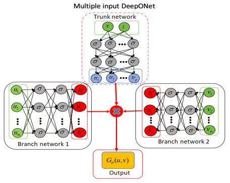
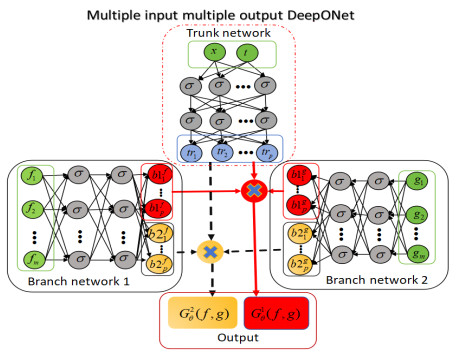
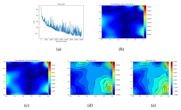
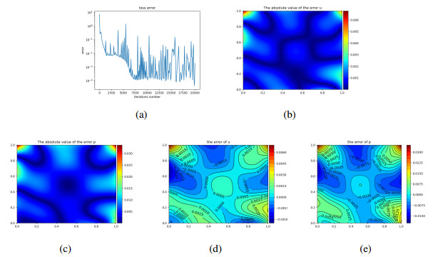
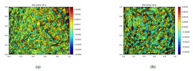
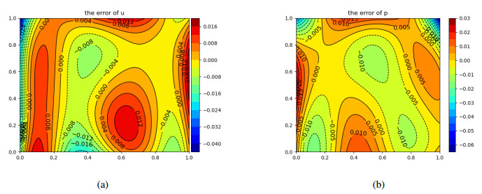
Deep operator networks is a popular machine learning approach. Some problems require multiple inputs and outputs. In this work, a multi-input and multi-output operator neural network (MIMOONet) for solving optimal control problems was proposed. To improve the accuracy of the numerical solution, a physics-informed MIMOONet was also proposed. To test the performance of the MIMOONet and the physics-informed MIMOONet, three examples, including elliptic (linear and semi-linear) and parabolic problems, were presented. The numerical results show that both methods are effective in solving these types of problems, and the physics-informed MIMOONet achieves higher accuracy due to its incorporation of physical laws.
- operator neural networks,
- multi-input,
- multi-output,
- physics-informed,
- PDE optimal control
Citation: Jinjun Yong, Xianbing Luo, Shuyu Sun. Deep multi-input and multi-output operator networks method for optimal control of PDEs[J]. Electronic Research Archive, 2024, 32(7): 4291-4320. doi: 10.3934/era.2024193

Related Papers:

Abstract

Deep operator networks is a popular machine learning approach. Some problems require multiple inputs and outputs. In this work, a multi-input and multi-output operator neural network (MIMOONet) for solving optimal control problems was proposed. To improve the accuracy of the numerical solution, a physics-informed MIMOONet was also proposed. To test the performance of the MIMOONet and the physics-informed MIMOONet, three examples, including elliptic (linear and semi-linear) and parabolic problems, were presented. The numerical results show that both methods are effective in solving these types of problems, and the physics-informed MIMOONet achieves higher accuracy due to its incorporation of physical laws.

References

[1]	G. Fabbri, Heat transfer optimization in corrugated wall channels, Int. J. Heat Mass Transfer, 43 (2000), 4299–4310. https://doi.org/10.1016/S0017-9310(00)00054-5 doi: 10.1016/S0017-9310(00)00054-5
[2]	G. Cornuéjols, J. Peña, R. Tütüncü, Optimization Methods in Finance, 2$^{nd}$, Cambridge University Press, New York, 2018.
[3]	J. C. De los Reyes, C. B. Schönlieb, Image denoising: learning the noise model via nonsmooth PDE-constrained optimization, Inverse Probl. Imaging, 7 (2013), 1183–1214. https://doi.org/10.3934/ipi.2013.7.1183 doi: 10.3934/ipi.2013.7.1183
[4]	J. Sokolowski, J. P. Zolésio, Introduction to Shape Optimization, Springer-Verlag, Berlin, 1992. https://doi.org/10.1007/978-3-642-58106-9_1
[5]	J. Haslinger, R. A. E. Mäkinen, Introduction to Shape Optimization: Theory, Approximation, and Computation, SIAM, Philadelphia, 2003. https://doi.org/10.1137/1.9780898718690
[6]	R. M. Hicks, P. A. Henne, Wing design by numerical optimization, J. Aircr., 15 (1978), 407–412. https://doi.org/10.2514/3.58379 doi: 10.2514/3.58379
[7]	P. D. Frank, G. R. Shubin, A comparison of optimization-based approaches for a model computational aerodynamics design problem, J. Comput. Phys., 98 (1992), 74–89. https://doi.org/10.1016/0021-9991(92)90174-W doi: 10.1016/0021-9991(92)90174-W
[8]	J. Ng, S. Dubljevic, Optimal boundary control of a diffusion-convection-reaction PDE model with time-dependent spatial domain: Czochralski crystal growth process, Chem. Eng. Sci., 67 (2012), 111–119. https://doi.org/10.1016/j.ces.2011.06.050 doi: 10.1016/j.ces.2011.06.050
[9]	S. P. Chakrabarty, F. B. Hanson, Optimal control of drug delivery to brain tumors for a distributed parameters model, in Proceedings of the 2005, American Control Conference, 2 (2005), 973–978. https://doi.org/10.1109/ACC.2005.1470086
[10]	W. B. Liu, N. N. Yan, Adaptive Finite Element Methods for Optimal Control Governed by PDEs, Science Press, Beijing, 2008.
[11]	Y. P. Chen, F. L. Huang, N. Yi, W. B. Liu, A Legendre Galerkin spectral method for optimal control problems governed by Stokes equations, SIAM J. Numer. Anal., 49 (2011), 1625–1648. https://doi.org/10.1137/080726057 doi: 10.1137/080726057
[12]	A. Borzì, V. Schulz, Computational Optimization of Systems Governed by Partial Differential Equations, SIAM, Philadelphia, 2011.
[13]	X. Luo, A priori error estimates of Crank-Nicolson finite volume element method for a hyperbolic optimal control problem, Numer. Methods Partial Differ. Equations, 32 (2016), 1331–1356. https://doi.org/10.1002/num.22052 doi: 10.1002/num.22052
[14]	M. Raissi, P. Perdikaris, G. E. Karniadakis, Physics informed deep learning (part Ⅰ): data-driven solutions of nonlinear partial differential equations, preprint, arXiv: 1711.10561.
[15]	S. Wang, H. Zhang, X. Jiang, Physics-informed neural network algorithm for solving forward and inverse problems of variable-order space-fractional advection-diffusion equations, Neurocomputing, 535 (2023), 64–82. https://doi.org/10.1016/j.neucom.2023.03.032 doi: 10.1016/j.neucom.2023.03.032
[16]	J. Sirignano, K. Spiliopoulos, DGM: a deep learning algorithm for solving partial differential equations, J. Comput. Phys., 375 (2018), 1339–1364. https://doi.org/10.1016/j.jcp.2018.08.029 doi: 10.1016/j.jcp.2018.08.029
[17]	W. N. E, B. Yu, The deep Ritz method: a deep-learning based numerical algorithm for solving variational problems, Commun. Math. Stat., 6 (2018), 1–12. https://doi.org/10.1007/s40304-018-0127-z doi: 10.1007/s40304-018-0127-z
[18]	Y. L. Liao, P. B. Ming, Deep Nitsche method: deep Ritz method with essential boundary conditions, Commun. Comput. Phys., 29 (2021), 1365–1384. https://doi.org/10.4208/cicp.OA-2020-0219 doi: 10.4208/cicp.OA-2020-0219
[19]	L. Lu, P. Z. Jin, G. F. Pang, Z. Q. Zhang, G. E. Karniadakis, Learning nonlinear operators via DeepONet based on the universal approximation theorem of operators, Nat. Mach. Intell., 3 (2021), 218–229. https://doi.org/10.1038/s42256-021-00302-5 doi: 10.1038/s42256-021-00302-5
[20]	C. Moya, S. Zhang, G. Lin, M. Yue, DeepONet-grid-UQ: a trustworthy deep operator framework for predicting the power grid's post-fault trajectories, Neurocomputing, 535 (2023), 166–182. https://doi.org/10.1016/j.neucom.2023.03.015 doi: 10.1016/j.neucom.2023.03.015
[21]	Z. Li, N. Kovachki, K. Azizzadenesheli, B. Liu, K. Bhattacharya, A. Stuart, et al., Neural operator: graph kernel network for partial differential equations, preprint, arXiv: 2003.03485.
[22]	Z. Li, N. Kovachki, K. Azizzadenesheli, B. Liu, K. Bhattacharya, A. Stuart, et al., Fourier neural operator for parametric partial differential equations, preprint, arXiv: 2010.08895.
[23]	S. F. Wang, H. W. Wang, P. Perdikaris, Learning the solution operator of parametric partial differential equations with physics-informed DeepOnets, Sci. Adv., 7 (2021), eabi8605. https://doi.org/10.1126/sciadv.abi8605 doi: 10.1126/sciadv.abi8605
[24]	P. Jin, S. Meng, L. Lu, MIONet: learning multiple-input operators via tensor product, SIAM J. Sci. Comput., 44 (2022), A3490–A3514. https://doi.org/10.1137/22M1477751 doi: 10.1137/22M1477751
[25]	C. J. García-Cervera, M. Kessler, F. Periago, Control of partial differential equations via physics-informed neural networks, J. Optim. Theory Appl., 196 (2023), 391–414. https://doi.org/10.1007/s10957-022-02100-4 doi: 10.1007/s10957-022-02100-4
[26]	S. Mowlavi, S. Nabib, Optimal control of PDEs using physics-informed neural networks, J. Comput. Phys., 473 (2023), 111731. https://doi.org/10.1016/j.jcp.2022.111731 doi: 10.1016/j.jcp.2022.111731
[27]	J. Barry-Straume, A. Sarsha, A. A. Popov, A. Sandu, Physics-informed neural networks for PDE-constrained optimization and control, preprint, arXiv: 2205.03377.
[28]	S. F. Wang, M. A. Bhouri, P. Perdikaris, Fast PDE-constrained optimization via self-supervised operator learning, preprint, arXiv: 2110.13297.
[29]	J.L. Lions, Optimal Control of Systems Governed by Partial Differential Equations, Springer-Verlag, Berlin, 1971.
[30]	T. P. Chen, H. Chen, Universal approximation to nonlinear operators by neural networks with arbitrary activation functions and its application to dynamical systems, IEEE Trans. Neural Networks, 6 (1995), 911–917. https://doi.org/10.1109/72.392253 doi: 10.1109/72.392253
[31]	I. Lasiecka, Mathematical Control Theory of Coupled PDEs, SIAM, Philadelphia, 2001. https://doi.org/10.1137/1.9780898717099
[32]	A. Miranville, The Cahn-Hilliard Equation: Recent Advances and Applications, SIAM, Philadelphia, 2019. https://doi.org/10.1137/1.9781611975925

Reader Comments

Your name:*

Email:*
© 2024 the Author(s), licensee AIMS Press. This is an open access article distributed under the terms of the Creative Commons Attribution License (http://creativecommons.org/licenses/by/4.0)