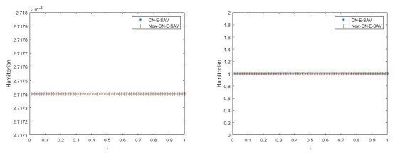
The keys to constructing numerical schemes for nonlinear partial differential equations are accuracy, handling of the nonlinear terms, and physical properties (energy dissipation or conservation). In this paper, we employ the exponential scalar auxiliary variable (E-SAV) method to solve a semi-linear wave equation. By defining two different variables and combining the Crank−Nicolson scheme, two semi-discrete schemes are proposed, both of which are second-order and maintain Hamiltonian conservation. Two numerical experiments are presented to verify the reliability of the theory.
Citation: Huanhuan Li, Lei Kang, Meng Li, Xianbing Luo, Shuwen Xiang. Hamiltonian conserved Crank-Nicolson schemes for a semi-linear wave equation based on the exponential scalar auxiliary variables approach[J]. Electronic Research Archive, 2024, 32(7): 4433-4453. doi: 10.3934/era.2024200
The keys to constructing numerical schemes for nonlinear partial differential equations are accuracy, handling of the nonlinear terms, and physical properties (energy dissipation or conservation). In this paper, we employ the exponential scalar auxiliary variable (E-SAV) method to solve a semi-linear wave equation. By defining two different variables and combining the Crank−Nicolson scheme, two semi-discrete schemes are proposed, both of which are second-order and maintain Hamiltonian conservation. Two numerical experiments are presented to verify the reliability of the theory.

| [1] | V. E. Zakharov, Exact solutions to the problem of the parametric interaction of three-dimensional wave packets, Sov. Phys. Dokl., 21 (1976). |
| [2] |
A. D. D. Craik, J. A. Adam, Evolution in space and time of resonant wave triads-Ⅰ. The'pump-wave approximation', Proc. R. Soc. Lond. A. Math. Phys. Sci., 363 (1978), 243–255. https://doi.org/10.1098/rspa.1978.0166 doi: 10.1098/rspa.1978.0166

|
| [3] |
I. Ahmed, A. R. Seadawy, D. Lu, Mixed lump-solitons, periodic lump and breather soliton solutions for (2+ 1)-dimensional extended Kadomtsev-Petviashvili dynamical equation, Int. J. Mod. Phys. B, 33 (2019), 1950019. https://doi.org/10.1142/S021797921950019X doi: 10.1142/S021797921950019X
|
| [4] |
Y. L. Ma, B. Q. Li, Interactions between soliton and rogue wave for a (2+1)-dimensional generalized breaking soliton system: hidden rogue wave and hidden soliton, Comput. Math. Appl., 78 (2019), 827–839. https://doi.org/10.1016/j.camwa.2019.03.002 doi: 10.1016/j.camwa.2019.03.002
|
| [5] |
A. Yusuf, T. A. Sulaiman, M. Inc, M. Bayram, Breather wave, lump-periodic solutions and some other interaction phenomena to the Caudrey-Dodd-Gibbon equation, Eur. Phys. J. Plus, 135 (2020), 1–8. https://doi.org/10.1140/epjp/s13360-020-00566-7 doi: 10.1140/epjp/s13360-020-00566-7
|
| [6] |
K. Hosseini, M. Samavat, M. Mirzazadeh, S. Salahshour, D. Baleanu, A new (4+1)-dimensional burgers equation: its backlund transformation and real and complex N-Kink solitons, Int. J. Appl. Comput. Math., 8 (2022), 172. https://doi.org/10.1007/s40819-022-01359-5 doi: 10.1007/s40819-022-01359-5
|
| [7] |
B. Q. Li, Y. L. Ma, Multiple-lump waves for a (3+1)-dimensional Boiti-Leon-Manna-Pempinelli equation arising from incompressible fluid, Comput. Math. Appl., 76 (2018), 204–214. https://doi.org/10.1016/j.camwa.2018.04.015 doi: 10.1016/j.camwa.2018.04.015
|
| [8] |
W. X. Ma, Riemann-Hilbert problems and soliton solutions of type (-$\lambda, \lambda$) reduced nonlocal integrable mKdV hierarchies, Mathematics, 10 (2022), 870. https://doi.org/10.3390/math10060870 doi: 10.3390/math10060870
|
| [9] |
Z. Zhao, L. He, M-lump, high-order breather solutions and interaction dynamics of a generalized (2+1)-dimensional nonlinear wave equation, Nonlinear Dyn., 100 (2020), 2753–2765. https://doi.org/10.1007/s11071-020-05611-9 doi: 10.1007/s11071-020-05611-9
|
| [10] |
J. G. Liu, M. S. Osman, Nonlinear dynamics for different nonautonomous wave structures solutions of a 3D variable-coefficient generalized shallow water wave equation, Chin. J. Phys., 77 (2022), 1618–1624. https://doi.org/10.1016/j.cjph.2021.10.026 doi: 10.1016/j.cjph.2021.10.026
|
| [11] |
U. Younas, T. A. Sulaiman, J. Ren, A. Yusuf, Lump interaction phenomena to the nonlinear ill-posed Boussinesq dynamical wave equation, J. Geom. Phys., 178 (2022), 104586. https://doi.org/10.1016/j.geomphys.2022.104586 doi: 10.1016/j.geomphys.2022.104586
|
| [12] |
H. F. Ismael, H. Bulut, M. S. Osman, The N-soliton, fusion, rational and breather solutions of two extensions of the (2+1)-dimensional Bogoyavlenskii-Schieff equation, Nonlinear Dyn., 107 (2022), 3791–3803. https://doi.org/10.1007/s11071-021-07154-z doi: 10.1007/s11071-021-07154-z
|
| [13] |
S. Saifullah, S. Ahmad, M. A. Alyami, M. Inc, Analysis of interaction of lump solutions with kink-soliton solutions of the generalized perturbed KdV equation using Hirota bilinear approach, Phys. Lett. A, 454 (2022), 128503. https://doi.org/10.1016/j.physleta.2022.128503 doi: 10.1016/j.physleta.2022.128503
|
| [14] |
Q. J. Feng, G. Q. Zhang, Lump solution, lump-stripe solution, rogue wave solution and periodic solution of the (2+1)-dimensional Fokas system, Nonlinear Dyn., 112 (2024), 4775–4792. https://doi.org/10.1007/s11071-023-09243-7 doi: 10.1007/s11071-023-09243-7
|
| [15] |
A. Degasperis, S. Lombardo, M. Sommacal, Integrability and linear stability of nonlinear waves, J. Nonlinear Sci., 28 (2018), 1251–1291. https://doi.org/10.1007/s00332-018-9450-5 doi: 10.1007/s00332-018-9450-5
|
| [16] |
M. J. Ablowitz, Integrability and nonlinear waves, Emerging Front. Nonlinear Sci., 32 (2020), 161–184. https://doi.org/10.1007/978-3-030-44992-6_7 doi: 10.1007/978-3-030-44992-6_7
|
| [17] |
M. He, P. Sun, Energy-preserving finite element methods for a class of nonlinear wave equations, Appl. Numer. Math., 157 (2020), 446–469. https://doi.org/10.1016/j.apnum.2020.06.016 doi: 10.1016/j.apnum.2020.06.016
|
| [18] |
M. He, J. Tian, P. Sun, Z. Zhang, An energy-conserving finite element method for nonlinear fourth-order wave equations, Appl. Numer. Math., 183 (2023), 333–354. https://doi.org/10.1016/j.apnum.2022.09.011 doi: 10.1016/j.apnum.2022.09.011
|
| [19] |
Y. Shi, X. Yang, Pointwise error estimate of conservative difference scheme for supergeneralized viscous Burgers equation, Electron. Res. Arch., 32 (2024), 1471–1497. https://doi.org/10.3934/era.2024068 doi: 10.3934/era.2024068
|
| [20] |
D. Furihata, Finite-difference schemes for nonlinear wave equation that inherit energy conservation property, J. Comput. Appl. Math., 134 (2001), 37–57. https://doi.org/10.1016/S0377-0427(00)00527-6 doi: 10.1016/S0377-0427(00)00527-6
|
| [21] |
Y. Liao, L. B. Liu, L. Ye, T. Liu, Uniform convergence analysis of the BDF2 scheme on Bakhvalov-type meshes for a singularly perturbed Volterra integro-differential equation, Appl. Math. Lett., 145 (2023), 108755. https://doi.org/10.1016/j.aml.2023.108755 doi: 10.1016/j.aml.2023.108755
|
| [22] |
Z. Zhou, H. Zhang, X. Yang, CN ADI fast algorithm on non-uniform meshes for the three-dimensional nonlocal evolution equation with multi-memory kernels in viscoelastic dynamics, Appl. Math. Comput., 474 (2024), 128680. https://doi.org/10.1016/j.amc.2024.128680 doi: 10.1016/j.amc.2024.128680
|
| [23] |
Y. O. Tijani A. R. Appadu, Unconditionally positive NSFD and classical finite difference schemes for biofilm formation on medical implant using Allen-Cahn equation, Demonstratio Math., 55 (2022), 40–60. https://doi.org/10.1515/dema-2022-0006 doi: 10.1515/dema-2022-0006
|
| [24] |
H. Zhang, X. Yang, Y. Liu, Y Liu, An extrapolated CN-WSGD OSC method for a nonlinear time fractional reaction-diffusion equation, Appl. Numer. Math., 157 (2020), 619–633. https://doi.org/10.1016/j.apnum.2020.07.017 doi: 10.1016/j.apnum.2020.07.017
|
| [25] |
X. Yang, Z. Zhang, Analysis of a new NFV scheme preserving DMP for two-dimensional sub-diffusion equation on distorted meshes, J. Sci. Comput., 99 (2024), 80. https://doi.org/10.1007/s10915-024-02511-7 doi: 10.1007/s10915-024-02511-7
|
| [26] |
S. F. Bradford, B. F. Sanders, Finite-volume models for unidirectional, nonlinear, dispersive waves, J. Waterw. Port. Coast., 128 (2002), 173–182. https://doi.org/10.1061/(ASCE)0733-950X(2002)128:4(173) doi: 10.1061/(ASCE)0733-950X(2002)128:4(173)
|
| [27] |
X. Yang, Z. Zhang, On conservative, positivity preserving, nonlinear FV scheme on distorted meshes for the multi-term nonlocal Nagumo-type equations, Appl. Math. Lett., 150 (2024), 108972. https://doi.org/10.1016/j.aml.2023.108972 doi: 10.1016/j.aml.2023.108972
|
| [28] | J. Shen, T. Tang, L. Wang, Spectral Methods: Algorithms, Analysis and Applications, Springer Science Business Media, 2011. |
| [29] |
M. Dehghan, A. Taleei, Numerical solution of nonlinear Schrödinger equation by using time-space-pseudo-spectral method, Numer. Meth. Part. Differ. Equations: Int. J., 26 (2010), 979–992. https://doi.org/10.1002/num.20468 doi: 10.1002/num.20468
|
| [30] |
T. Lu, W. Cai, A Fourier spectral-discontinuous Galerkin method for time-dependent 3-D Schrödinger-Poisson equations with discontinuous potentials, J. Comput. Appl. Math., 220 (2008), 588–614. https://doi.org/10.1016/j.cam.2007.09.025 doi: 10.1016/j.cam.2007.09.025
|
| [31] |
Y. Shi, X. Yang, A time two-grid difference method for nonlinear generalized viscous Burgers equation, J. Math. Chem., 62 (2024), 1323–1356. https://doi.org/10.1007/s10910-024-01592-x doi: 10.1007/s10910-024-01592-x
|
| [32] |
M. Yao, Z. Weng, A numerical method based on operator splitting collocation scheme for nonlinear Schrödinger equation, Math. Comput. Appl., 29 (2024), 6. https://doi.org/10.3390/mca29010006 doi: 10.3390/mca29010006
|
| [33] |
K. J. Ansari, M. Izadi, S. Noeiaghdam, Enhancing the accuracy and efficiency of two uniformly convergent numerical solvers for singularly perturbed parabolic convection- diffusion-reaction problems with two small parameters, Demonstratio Math., 57 (2024), 20230144. https://doi.org/10.1515/dema-2023-0144 doi: 10.1515/dema-2023-0144
|
| [34] |
Z. Guan, C. Wang, S. M. Wise, A convergent convex splitting scheme for the periodic nonlocal Cahn-Hilliard equation, Numer. Math., 128 (2014), 377–406. https://doi.org/10.1007/s00211-014-0608-2 doi: 10.1007/s00211-014-0608-2
|
| [35] |
Z. Guan, J. S. Lowengrub, C. Wang, S. M. Wise, Second order convex splitting schemes for periodic nonlocal Cahn-Hilliard and Allen-Cahn equations, J. Comput. Phys., 277 (2014), 48–71. https://doi.org/10.1016/j.jcp.2014.08.001 doi: 10.1016/j.jcp.2014.08.001
|
| [36] |
J. Shen, C. Wang, X. Wang, S. M. Wise, Second-order convex splitting schemes for gradient flows with Ehrlich-Schwoebel type energy: application to thin film epitaxy, SIAM J. Numer. Anal., 50 (2012), 105–125. https://doi.org/10.1137/110822839 doi: 10.1137/110822839
|
| [37] |
X. Feng, T. Tang, J. Yang, Stabilized Crank-Nicolson/Adams-Bashforth schemes for phase field models, East Asian J. Appl. Math., 3 (2013), 59–80. https://doi.org/10.4208/eajam.200113.220213a doi: 10.4208/eajam.200113.220213a
|
| [38] |
J. Shen, X. Yang, Numerical approximations of Allen-Cahn and Cahn-Hilliard equations, Discrete Contin. Dyn. Syst., 28 (2010), 1669–1691. https://doi.org/10.3934/dcds.2010.28.1669 doi: 10.3934/dcds.2010.28.1669
|
| [39] |
L. Ju, X. Li, Z. Qiao, H. Zhang, Energy stability and error estimates of exponential time differencing schemes for the epitaxial growth model without slope selection, Math. Comput., 87 (2018), 1859-1885. https://doi.org/10.1090/mcom/3262 doi: 10.1090/mcom/3262
|
| [40] |
L. Ju, J. Zhang, Q. Du, Fast and accurate algorithms for simulating coarsening dynamics of Cahn-Hilliard equations, Comput. Mater. Sci., 108 (2015), 272–282. https://doi.org/10.1016/j.commatsci.2015.04.046 doi: 10.1016/j.commatsci.2015.04.046
|
| [41] |
J. Zhao, Q. Wang, X. Yang, Numerical approximations for a phase field dendritic crystal growth model based on the invariant energy quadratization approach, Int. J. Numer. Meth. Eng., 110 (2017), 279–300. https://doi.org/10.1002/nme.5372 doi: 10.1002/nme.5372
|
| [42] |
J. Shen, J. Xu, Convergence and error analysis for the scalar auxiliary variable (SAV) schemes to gradient flows, SIAM J. Numer. Anal., 56 (2018), 2895–2912. https://doi.org/10.1137/17M1159968 doi: 10.1137/17M1159968
|
| [43] |
J. Shen, J. Xu, J. Yang, A new class of efficient and robust energy stable schemes for gradient flows, SIAM Rev., 61 (2019), 474–506. https://doi.org/10.1137/17M1150153 doi: 10.1137/17M1150153
|
| [44] |
Z. Liu, X. Li, The exponential scalar auxiliary variable (E-SAV) approach for phase field models and its explicit computing, SIAM J. Sci. Comput., 42 (2020), B630–B655. https://doi.org/10.1137/19M1305914 doi: 10.1137/19M1305914
|
| [45] |
F. Huang, J. Shen, Z. Yang, A highly efficient and accurate new scalar auxiliary variable approach for gradient flows, SIAM J. Sci. Comput., 42 (2020), A2514–A2536. https://doi.org/10.1137/19M1298627 doi: 10.1137/19M1298627
|
| [46] |
Z. Liu, X. Li, A highly efficient and accurate exponential semi-implicit scalar auxiliary variable (ESI-SAV) approach for dissipative system, J. Comput. Phys., 447 (2021), 110703. https://doi.org/10.1016/j.jcp.2021.110703 doi: 10.1016/j.jcp.2021.110703
|
| [47] |
C. Jiang, W. Cai, Y. Wang, A linearly implicit and local energy-preserving scheme for the sine-Gordon equation based on the invariant energy quadratization approach, J. Sci. Comput., 80 (2019), 1629–1655. https://doi.org/10.1007/s10915-019-01001-5 doi: 10.1007/s10915-019-01001-5
|
| [48] |
D. Li, W. Sun, Linearly implicit and high-order energy-conserving schemes for nonlinear wave equations, J. Sci. Comput., 83 (2020), 1–17. https://doi.org/10.1007/s10915-020-01245-6 doi: 10.1007/s10915-020-01245-6
|
| [49] |
N. Wang, M. Li, C. Huang, Unconditional energy dissipation and error estimates of the SAV Fourier Spectral Method for nonlinear fractional generalized wave equation, J. Sci. Comput., 88 (2021), 19. https://doi.org/10.1007/s10915-021-01534-8 doi: 10.1007/s10915-021-01534-8
|
| [50] |
F. Yu, M. Chen, Error analysis of the Crank-Nicolson SAV method for the Allen-Cahn equation on variable grids, Appl. Math. Lett., 125 (2022), 107768. https://doi.org/10.1016/j.aml.2021.107768 doi: 10.1016/j.aml.2021.107768
|
| [51] |
L. Ju, X. Li, Z. Qiao, Stabilized exponential-SAV schemes preserving energy dissipation law and maximum bound principle for the Allen-Cahn type equations, J. Sci. Comput., 92 (2022), 66. https://doi.org/10.1007/s10915-022-01921-9 doi: 10.1007/s10915-022-01921-9
|
Figures(1) / Tables(6)
Huanhuan Li, Lei Kang, Meng Li, Xianbing Luo, Shuwen Xiang. Hamiltonian conserved Crank-Nicolson schemes for a semi-linear wave equation based on the exponential scalar auxiliary variables approach[J]. Electronic Research Archive, 2024, 32(7): 4433-4453. doi: 10.3934/era.2024200


 DownLoad: