Epidemiologists have used the timing of the peak of an epidemic to guide public health interventions. By determining the expected peak time, they can allocate resources effectively and implement measures such as quarantine, vaccination, and treatment at the right time to mitigate the spread of the disease. The peak time also provides valuable information for those modeling the spread of the epidemic and making predictions about its future trajectory. In this study, we analyze the time needed for an epidemic to reach its peak by presenting a straightforward analytical expression. Utilizing two epidemiological models, the first is a generalized $ SEIR $ model with two classes of latent individuals, while the second incorporates a continuous age structure for latent infections. We confirm the conjecture that the peak occurs at approximately $ T\sim(\ln N)/\lambda $, where $ N $ is the population size and $ \lambda $ is the largest eigenvalue of the linearized system in the first model or the unique positive root of the characteristic equation in the second model. Our analytical results are compared to numerical solutions and shown to be in good agreement.
Citation: Ali Moussaoui, Mohammed Meziane. On the date of the epidemic peak[J]. Mathematical Biosciences and Engineering, 2024, 21(2): 2835-2855. doi: 10.3934/mbe.2024126
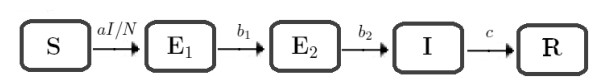
Epidemiologists have used the timing of the peak of an epidemic to guide public health interventions. By determining the expected peak time, they can allocate resources effectively and implement measures such as quarantine, vaccination, and treatment at the right time to mitigate the spread of the disease. The peak time also provides valuable information for those modeling the spread of the epidemic and making predictions about its future trajectory. In this study, we analyze the time needed for an epidemic to reach its peak by presenting a straightforward analytical expression. Utilizing two epidemiological models, the first is a generalized $ SEIR $ model with two classes of latent individuals, while the second incorporates a continuous age structure for latent infections. We confirm the conjecture that the peak occurs at approximately $ T\sim(\ln N)/\lambda $, where $ N $ is the population size and $ \lambda $ is the largest eigenvalue of the linearized system in the first model or the unique positive root of the characteristic equation in the second model. Our analytical results are compared to numerical solutions and shown to be in good agreement.

| [1] | R. M. Anderson, R. M. May, Infectious Diseases of Humans: Dynamics and Control, Oxford University Press, 1991. |
| [2] |
M. Koivu-Jolma, A. Annila, Epidemic as a natural process, Math. Biosci., 299 (2018), 0025–5564. https://doi.org/10.1016/j.mbs.2018.03.012 doi: 10.1016/j.mbs.2018.03.012

|
| [3] |
M. De la Sen, R. Nistal, A. Ibeas, A. J. Garrido, On the use of entropy issues to evaluate and control the transients in some epidemic models, Entropy, 22 (2020), 534. https://doi.org/10.3390/e22050534 doi: 10.3390/e22050534
|
| [4] |
T. Nguyen-Huu, P. Auger, A. Moussaoui, On incidence-dependent management strategies against an SEIRS epidemic: Extinction of the epidemic using allee effect, Mathematics, 11 (2023), 2822. https://doi.org/10.3390/math11132822 doi: 10.3390/math11132822
|
| [5] |
S. Fisher-Hoch, L. Hutwagner, Opportunistic candidiasis: An epidemic of the 1980s, Clin. Infect. Dis., 21 (1995), 897–904. https://doi.org/10.1093/clinids/21.4.897 doi: 10.1093/clinids/21.4.897
|
| [6] |
C. Chintu, U. H. Athale, P. Patil, Childhood cancers in Zambia before and after the HIV epidemic, Arch. Dis. Child., 73 (1995), 100–105. https://doi.org/10.1136/adc.73.2.100 doi: 10.1136/adc.73.2.100
|
| [7] |
R. M. Anderson, C. Fraser, A. C. Ghani, C. A. Donnelly, S. Riley, N. M. Ferguson, et al., Epidemiology, transmission dynamics and control of SARS: The 2002–2003 epidemic, Philos. Trans. R. Soc. London Ser. B: Biol. Sci., 359 (2004), 1091–1105. https://doi.org/10.1098/rstb.2004.1490 doi: 10.1098/rstb.2004.1490
|
| [8] |
W. Lam, N. Zhong, W. Tan, Overview on sars in asia and the world, Respirology, 8 (2003), S2–S5. https://doi.org/10.1046/j.1440-1843.2003.00516.x doi: 10.1046/j.1440-1843.2003.00516.x
|
| [9] |
W. Wang, Z. Wu, C. Wang, R. Hu, Modelling the spreading rate of controlled communicable epidemics through an entropy-based thermodynamic model, Sci. China Phys. Mech. Astron., 56 (2013), 2143–2150. https://doi.org/10.1007/s11433-013-5321-0 doi: 10.1007/s11433-013-5321-0
|
| [10] |
H. Chen, G. Smith, K. Li, J. Wang, X. Fan, J. Rayner, et al., Establishment of multiple sublineages of H5N1 influenza virus in Asia: implications for pandemic control, Proc. Natl. Acad. Sci., 103 (2006), 2845–2850. https://doi.org/10.1073/pnas.0511120103 doi: 10.1073/pnas.0511120103
|
| [11] |
A. M. Kilpatrick, A. A. Chmura, D. W. Gibbons, R. C. Fleischer, P. P. Marra, P. Daszak, Predicting the global spread of h5n1 avian influenza, Proc. Natl. Acad. Sci., 103 (2006), 19368–19373. https://doi.org/10.1073/pnas.0609227103 doi: 10.1073/pnas.0609227103
|
| [12] |
S. Jain, L. Kamimoto, A. M. Bramley, A. M. Schmitz, S. R. Benoit, J. Louie, et al., Hospitalized patients with 2009 H1N1 influenza in the United States, April–June 2009, N. Engl. J. Med., 361 (2009), 1935–1944. https://doi.org/10.1056/NEJMoa0906695 doi: 10.1056/NEJMoa0906695
|
| [13] |
M. P. Girard, J. S. Tam, O. M. Assossou, M. P. Kieny, The 2009 A (H1N1) influenza virus pandemic: A review, Vaccine, 28 (2010), 4895–4902. https://doi.org/10.1016/j.vaccine.2010.05.031 doi: 10.1016/j.vaccine.2010.05.031
|
| [14] |
T. R. Frieden, I. Damon, B. P. Bell, T. Kenyon, S. Nichol, Ebola 2014–new challenges, new global response and responsibility, N. Engl. J. Med., 371 (2014), 1177–1180. https://doi.org/10.1056/NEJMp1409903 doi: 10.1056/NEJMp1409903
|
| [15] |
W. E. R. Team, Ebola virus disease in West Africa-the first 9 months of the epidemic and forward projections, N. Engl. J. Med., 371 (2014), 1481–1495. https://doi.org/10.1056/NEJMoa1411100 doi: 10.1056/NEJMoa1411100
|
| [16] |
A. Moussaoui, E. H. Zerga, Transmission dynamics of COVID-19 in Algeria: The impact of physical distancing and face masks, AIMS Public Health, 7 (2020), 816. https://doi.org/10.3934/publichealth.2020063 doi: 10.3934/publichealth.2020063
|
| [17] |
P. Auger, A. Moussaoui, On the threshold of release of confinement in an epidemic SEIR model taking into account the protective effect of mask, Bull. Math. Biol., 83 (2021), 25. https://doi.org/10.1007/s11538-021-00858-8 doi: 10.1007/s11538-021-00858-8
|
| [18] |
A. Moussaoui, P. Auger, Prediction of confinement effects on the number of COVID-19 outbreak in Algeria, Math. Modell. Nat. Phenom., 15 (2020), 37. https://doi.org/10.1051/mmnp/2020028 doi: 10.1051/mmnp/2020028
|
| [19] |
M. Meziane, A. Moussaoui, V. Vitaly, On a two-strain epidemic model involving delay equations, Math. Biosci. Eng., 20 (2020), 20683–20711. https://doi.org/10.3934/mbe.2023915 doi: 10.3934/mbe.2023915
|
| [20] | N. Bacaër, Mathématiques et épidémies, Cassini, 212 (2021). |
| [21] |
M. Turkyilmazoglu, Explicit formulae for the peak time of an epidemic from the sir model, Phys. D: Nonlinear Phenom., 422 (2021), 132902. https://doi.org/10.1016/j.physd.2021.132902 doi: 10.1016/j.physd.2021.132902
|
| [22] |
M. Turkyilmazoglu, A highly accurate peak time formula of epidemic outbreak from the SIR model, Chin. J. Phys., 84 (2023), 39–50. https://doi.org/10.1016/j.cjph.2023.05.009 doi: 10.1016/j.cjph.2023.05.009
|
| [23] |
N. Piovella, Analytical solution of seir model describing the free spread of the covid-19 pandemic, Chaos, Solitons Fractals, 140 (2020), 110243. https://doi.org/10.1016/j.chaos.2020.110243 doi: 10.1016/j.chaos.2020.110243
|
| [24] |
N. Bame, S. Bowong, J. Mbang, G. Sallet, J. J. Tewa, Global stability analysis for SEIS models with n latent classes, Math. Biosci. Eng., 5 (2008), 20–33. https://doi.org/10.3934/mbe.2008.5.20 doi: 10.3934/mbe.2008.5.20
|
| [25] |
S. Sharma, V. Volpert, M. Banerjee, Extended SEIQR type model for COVID-19 epidemic and data analysis, Math. Biosci. Eng., 17 (2020), 7562–7604. https://doi.org/10.3934/mbe.2020386 doi: 10.3934/mbe.2020386
|
| [26] |
O. Diekmann, J. A. P. Heesterbeek, J. A. Metz, On the definition and the computation of the basic reproduction ratio r 0 in models for infectious diseases in heterogeneous populations, J. Math. Biol., 28 (1990), 365–382. https://doi.org/10.1007/BF00178324 doi: 10.1007/BF00178324
|
| [27] |
P. Van den Driessche, J. Watmough, Reproduction numbers and sub-threshold endemic equilibria for compartmental models of disease transmission, Math. Biosci., 180 (2002), 29–48. https://doi.org/10.1016/S0025-5564(02)00108-6 doi: 10.1016/S0025-5564(02)00108-6
|
| [28] | L. Perko, Differential Equations and Dynamical Systems, 3rd Edition, Springer Science Business Media, 7 (2013). https://doi.org/10.1007/978-1-4613-0003-8 |
| [29] |
H. L. Smith, Monotone dynamical systems: an introduction to the theory of competitive and cooperative systems: An introduction to the theory of competitive and cooperative systems, Am. Math. Soc., 41 (2008). http://dx.doi.org/10.1090/surv/041 doi: 10.1090/surv/041
|
| [30] |
M. W. Hirsch, Systems of differential equations that are competitive or cooperative ii: Convergence almost everywhere, SIAM J. Math. Anal., 16 (1985), 423–439. https://doi.org/10.1137/0516030 doi: 10.1137/0516030
|
| [31] | H. R. Thieme, Mathematics in Population Biology, Princeton University Press, 12 (1985). https://doi.org/10.1515/9780691187655 |
| [32] |
A. Berman, R. J. Plemmons, Nonnegative matrices in the mathematical sciences, Soc. Ind. Appl. Math., 1994. https://doi.org/10.1137/1.9781611971262 doi: 10.1137/1.9781611971262
|
| [33] |
J. É. Rombaldi, Analyse matricielle-Cours et exercices résolus: 2e édition, EDP Sci., 2019. https://doi.org/10.1051/978-2-7598-2419-9.toc doi: 10.1051/978-2-7598-2419-9.toc
|
| [34] |
C. Van Loan, The sensitivity of the matrix exponential, SIAM J. Math. Anal., 14 (1977), 971–981. https://doi.org/10.1137/0714065 doi: 10.1137/0714065
|
| [35] | H. Brezis, Analyse fonctionnelle, Théorie et Applications, 1983. |
| [36] | H. K. Khalil, Nonlinear Systems, 3rd edition, Patience Hall, 115 (2002). |


Figures(3)

Ali Moussaoui, Mohammed Meziane. On the date of the epidemic peak[J]. Mathematical Biosciences and Engineering, 2024, 21(2): 2835-2855. doi: 10.3934/mbe.2024126


 DownLoad: