Semi-supervised medical image segmentation is currently a highly researched area. Pseudo-label learning is a traditional semi-supervised learning method aimed at acquiring additional knowledge by generating pseudo-labels for unlabeled data. However, this method relies on the quality of pseudo-labels and can lead to an unstable training process due to differences between samples. Additionally, directly generating pseudo-labels from the model itself accelerates noise accumulation, resulting in low-confidence pseudo-labels. To address these issues, we proposed a dual uncertainty-guided multi-model pseudo-label learning framework (DUMM) for semi-supervised medical image segmentation. The framework consisted of two main parts: The first part is a sample selection module based on sample-level uncertainty (SUS), intended to achieve a more stable and smooth training process. The second part is a multi-model pseudo-label generation module based on pixel-level uncertainty (PUM), intended to obtain high-quality pseudo-labels. We conducted a series of experiments on two public medical datasets, ACDC2017 and ISIC2018. Compared to the baseline, we improved the Dice scores by 6.5% and 4.0% over the two datasets, respectively. Furthermore, our results showed a clear advantage over the comparative methods. This validates the feasibility and applicability of our approach.
Citation: Zhanhong Qiu, Weiyan Gan, Zhi Yang, Ran Zhou, Haitao Gan. Dual uncertainty-guided multi-model pseudo-label learning for semi-supervised medical image segmentation[J]. Mathematical Biosciences and Engineering, 2024, 21(2): 2212-2232. doi: 10.3934/mbe.2024097
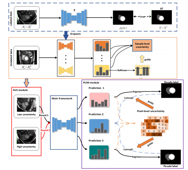
Semi-supervised medical image segmentation is currently a highly researched area. Pseudo-label learning is a traditional semi-supervised learning method aimed at acquiring additional knowledge by generating pseudo-labels for unlabeled data. However, this method relies on the quality of pseudo-labels and can lead to an unstable training process due to differences between samples. Additionally, directly generating pseudo-labels from the model itself accelerates noise accumulation, resulting in low-confidence pseudo-labels. To address these issues, we proposed a dual uncertainty-guided multi-model pseudo-label learning framework (DUMM) for semi-supervised medical image segmentation. The framework consisted of two main parts: The first part is a sample selection module based on sample-level uncertainty (SUS), intended to achieve a more stable and smooth training process. The second part is a multi-model pseudo-label generation module based on pixel-level uncertainty (PUM), intended to obtain high-quality pseudo-labels. We conducted a series of experiments on two public medical datasets, ACDC2017 and ISIC2018. Compared to the baseline, we improved the Dice scores by 6.5% and 4.0% over the two datasets, respectively. Furthermore, our results showed a clear advantage over the comparative methods. This validates the feasibility and applicability of our approach.

| [1] | O. Ronneberger, P. Fischer, T. Brox, U-net: Convolutional networks for biomedical image segmentation, in Medical Image Computing and Computer-Assisted Intervention–MICCAI 2015: 18th International Conference, Munich, Germany, October 5–9, 2015, Proceedings, Part III 18, (2015), 234–241. https://doi.org/10.1007/978331924574428 |
| [2] | F. Milletari, N. Navab, S. Ahmadi, V-net: Fully convolutional neural networks for volumetric medical image segmentation, in 2016 Fourth International Conference on 3D Vision (3DV), (2016), 565–571. https://doi.org/10.1109/3DV.2016.79 |
| [3] |
L. Qiu, H. Ren, RSegNet: A joint learning framework for deformable registration and segmentation, IEEE Trans. Autom. Sci. Eng., 19 (2021), 2499–2513. https://doi.org/10.1109/TASE.2021.3087868 doi: 10.1109/TASE.2021.3087868

|
| [4] |
W. Kim, A. Kanezaki, M. Tanaka, Unsupervised learning of image segmentation based on differentiable feature clustering, IEEE Trans. Image Process., 29 (2020), 8055–8068. https://doi.org/10.1109/TIP.2020.3011269 doi: 10.1109/TIP.2020.3011269
|
| [5] |
W. Lei, Q. Su, T. Jiang, R. Gu, N. Wang, X. Liu, et al., One-shot weakly-supervised segmentation in 3D medical images, IEEE Trans. Med. Imaging, 43 (2024), 175–189. https://doi.org/10.1109/TMI.2023.3294975 doi: 10.1109/TMI.2023.3294975
|
| [6] | D. H. Lee, Pseudo-label: The simple and efficient semi-supervised learning method for deep neural networks, in Workshop on Challenges in Representation Learning, ICML, 3 (2013), 896. https://doi.org/10.1007/978331966185829 |
| [7] | W. Bai, O. Oktay, M. Sinclair, H. Suzuki, M. Rajchl, G. Tarroni, et al., Semi-supervised learning for network-based cardiac MR image segmentation, in Medical Image Computing and Computer-Assisted Intervention-MICCAI 2017: 20th International Conference, Quebec City, QC, Canada, September 11–13, 2017, Proceedings, Part II 20, (2017), 253–260. https://doi.org/10.1007/978-3-030-32248-9_51 |
| [8] | N. Srivastava, G. Hinton, A. Krizhevsky, I. Sutskever, R. Salakhutdinov, Dropout: a simple way to prevent neural networks from overfitting, J. Mach. Learn. Res., 15 (2014), 1929–1958. |
| [9] | S. Chen, G. Bortsova, A. Garcia-Uceda Juarez, G. Van Tulder, M. De Bruijne, Multi-task attention-based semi-supervised learning for medical image segmentation, in Medical Image Computing and Computer Assisted Intervention–MICCAI 2019: 22nd International Conference, Shenzhen, China, October 13–17, 2019, Proceedings, Part III 22, (2019), 457–465. https://doi.org/10.1007/978303032248951 |
| [10] | L. Sun, J. Wu, X. Ding, Y. Huang, G. Wang, Y. Yu, A teacher-student framework for semi-supervised medical image segmentation from mixed supervision, preprint, arXiv: 2010.12219. https://doi.org/10.48550/arXiv.2010.12219 |
| [11] |
X. Luo, G. Wang, W. Liao, J. Chen, T. Song, Y. Chen, et al., Semi-supervised medical image segmentation via uncertainty rectified pyramid consistency, Med. Image Anal., 80 (2022), 102517. https://doi.org/10.1016/j.media.2022.102517 doi: 10.1016/j.media.2022.102517
|
| [12] |
Y. Wu, Z. Ge, D. Zhang, M. Xu, L. Zhang, Y. Xia, et al., Mutual consistency learning for semi-supervised medical image segmentation, Med. Image Anal., 81 (2022), 102530. https://doi.org/10.1016/j.media.2022.102530 doi: 10.1016/j.media.2022.102530
|
| [13] |
Y. Xie, J. Zhang, Z. Liao, J. Verjans, C. Shen, Y. Xia, Intra-and inter-pair consistency for semi-supervised gland segmentation, IEEE Trans. Image Process., 31 (2021), 894–905. https://doi.org/10.1109/TIP.2021.3136716 doi: 10.1109/TIP.2021.3136716
|
| [14] |
C. Chen, K. Zhou, Z. Wang, R. Xiao, Generative consistency for semi-supervised cerebrovascular segmentation from TOF-MRA, IEEE Trans. Med. Imaging, 42 (2022), 346–353. https://doi.org/10.1109/TMI.2022.3184675 doi: 10.1109/TMI.2022.3184675
|
| [15] | A. Tarvainen, H. Valpola, Mean teachers are better role models: Weight-averaged consistency targets improve semi-supervised deep learning results, in Advances in Neural Information Processing Systems, 30 (2017). |
| [16] |
Y. Zhang, R. Jiao, Q. Liao, D. Li, J. Zhang, Uncertainty-guided mutual consistency learning for semi-supervised medical image segmentation, Artif. Intell. Med., 138 (2023), 102476. https://doi.org/10.1016/j.artmed.2022.102476 doi: 10.1016/j.artmed.2022.102476
|
| [17] |
K. Wang, B. Zhan, C. Zu, X. Wu, J. Zhou, L. Zhou, et al., Semi-supervised medical image segmentation via a tripled-uncertainty guided mean teacher model with contrastive learning, Med. Image Anal., 79 (2022), 102447. https://doi.org/10.1016/j.media.2022.102447 doi: 10.1016/j.media.2022.102447
|
| [18] | Z. Qiu, H. Gan, M. Shi, Z. Huang, Z. Yang, Self-training with dual uncertainty for semi-supervised medical image segmentation, preprint, arXiv: 2304.04441. https://doi.org/10.48550/arXiv.2304.04441 |
| [19] | K. Sohn, D. Berthelot, N. Carlini, Z. Zhang, H. Zhang, C. Raffel, et al., Fixmatch: Simplifying semi-supervised learning with consistency and confidence, in Advances in Neural Information Processing Systems, 33 (2020), 596–608. |
| [20] | D. Berthelot, N. Carlini, I. Goodfellow, N. Papernot, A. Oliver, C. A. Raffel, Mixmatch: A holistic approach to semi-supervised learning, in Advances in Neural Information Processing Systems, 32 (2019). |
| [21] | A. Kurakin, C. Raffel, D. Berthelot, E. D. Cubuk, H. Zhang, K. Sohn, et al., Remixmatch: Semi-supervised learning with distribution matching and augmentation anchoring, 2020. Available from: https://research.google/pubs/remixmatch-semi-supervised-learning-with-distribution-matching-and-augmentation-anchoring/. |
| [22] | S. Laine, T. Aila, Temporal ensembling for semi-supervised learning, preprint, arXiv: 1610.02242. https://doi.org/10.48550/arXiv.1610.02242 |
| [23] | J. Li, C. Xiong, S. Hoi, Comatch: Semi-supervised learning with contrastive graph regularization, in Proceedings of the IEEE/CVF International Conference on Computer Vision, (2021), 9475–9484. |
| [24] | M. Zheng, S. You, L. Huang, F. Wang, C. Qian, C. Xu, Simmatch: Semi-supervised learning with similarity matching, in Proceedings of the IEEE/CVF Conference on Computer Vision and Pattern Recognition, (2022), 14471–14481. |
| [25] | W. J. Maddox, P. Izmailov, T. Garipov, D. P. Vetrov, A. G. Wilson, A simple baseline for bayesian uncertainty in deep learning, in Advances in Neural Information Processing Systems, 32 (2019). |
| [26] | M. N. Rizve, K. Duarte, Y. S. Rawat, M. Shah, In defense of pseudo-labeling: An uncertainty-aware pseudo-label selection framework for semi-supervised learning, preprint, arXiv: 2101.06329. https://doi.org/10.48550/arXiv.2101.06329 |
| [27] | L. Yu, S. Wang, X. Li, C. W. Fu, P. A. Heng, Uncertainty-aware self-ensembling model for semi-supervised 3D left atrium segmentation, in Medical Image Computing and Computer Assisted Intervention–MICCAI 2019: 22nd International Conference, Shenzhen, China, October 13–17, 2019, Proceedings, Part II 22, (2019), 605–613. https://doi.org/10.1007/978303032245867 |
| [28] | J. Fan, B. Gao, H. Jin, L. Jiang, Ucc: Uncertainty guided cross-head co-training for semi-supervised semantic segmentation, in Proceedings of the IEEE/CVF Conference on Computer Vision and Pattern Recognition, (2022), 9947–9956. |
| [29] | Z. Shen, P. Cao, H. Yang, X. Liu, J. Yang, O. R. Zaiane, Co-training with high-confidence Pseudo labels for semi-supervised medical image segmentation, preprint, arXiv: 2301.04465. https://doi.org/10.48550/arXiv.2301.04465 |
| [30] | Z. Xu, J. Luo, D. Lu, J. Yan, S. Frisken, J. Jagadeesan, et al., Double-uncertainty guided spatial and temporal consistency regularization weighting for learning-based abdominal registration, in International Conference on Medical Image Computing and Computer-Assisted Intervention, (2022), 14–24. |
| [31] | J. Zhang, J. Lyu, X. Ma, J. Yan, J. Yang, L. Wan, et al., Uncertainty-driven trajectory truncation for model-based offline reinforcement learning, preprint, arXiv: 2304.04660. https://doi.org/10.48550/arXiv.2304.04660 |
| [32] |
X. Wang, Y. Yuan, D. Guo, X. Huang, Y. Cui, M. Xia, et al., SSA-Net: Spatial self-attention network for COVID-19 pneumonia infection segmentation with semi-supervised few-shot learning, Med. Image Anal., 79 (2022), 102459. https://doi.org/10.1016/j.media.2022.102459 doi: 10.1016/j.media.2022.102459
|
| [33] |
Y. Shi, J. Zhang, T. Ling, J. Lu, Y. Zheng, Q. Yu, et al., Inconsistency-aware uncertainty estimation for semi-supervised medical image segmentation, IEEE Trans. Med. Imaging, 41 (2021), 608–620. https://doi.org/10.1109/TMI.2021.3117888 doi: 10.1109/TMI.2021.3117888
|
| [34] | Y. Zhang, B. Zhou, L. Chen, Y. Wu, H. Zhou, Multi-transformation consistency regularization for semi-supervised medical image segmentation, in 2021 4th International Conference on Artificial Intelligence and Big Data (ICAIBD), (2021), 485–489. https://doi.org/10.1109/ICAIBD51990.2021.9459059 |
| [35] | H. Basak, R. Bhattacharya, R. Hussain, A. Chatterjee, An embarrassingly simple consistency regularization method for semi-supervised medical image segmentation, preprint, arXiv: 2202.00677. https://doi.org/10.48550/arXiv.2202.00677 |
| [36] | H. Basak, Z. Yin, Pseudo-label guided contrastive learning for semi-supervised medical image segmentation, in Proceedings of the IEEE/CVF Conference on Computer Vision and Pattern Recognition, (2023), 19786–19797. |
| [37] | Y. Bai, D. Chen, Q. Li, W. Shen, Y. Wang, Bidirectional copy-paste for semi-supervised medical image segmentation, in Proceedings of the IEEE/CVF Conference on Computer Vision and Pattern Recognition, (2023), 11514–11524. |
| [38] | Z. Xu, D. Lu, J. Yan, J. Sun, J. Luo, D. Wei, et al., Category-level regularized unlabeled-to-labeled learning for semi-supervised prostate segmentation with multi-site unlabeled data, in International Conference on Medical Image Computing and Computer-Assisted Intervention, (2023), 3–13. https://doi.org/10.1007/97830314390181 |
| [39] | W. Pan, J. Yan, H. Chen, J. Yang, Z. Xu, X. Li, et al., Human-machine interactive tissue prototype learning for label-efficient histopathology image segmentation, in International Conference on Medical Image Computing and Computer-Assisted Intervention, (2023), 3–13. https://doi.org/10.1007/978303134048252 |
| [40] |
J. Peng, G. Estrada, M. Pedersoli, C. Desrosiers, Deep co-training for semi-supervised image segmentation, Pattern Recognit., 107 (2020), 107269. https://doi.org/10.1016/j.patcog.2020.107269 doi: 10.1016/j.patcog.2020.107269
|
| [41] | L. Yang, W. Zhuo, L. Qi, Y. Shi, Y. Gao, ST++: Make self-training work better for semi-supervised semantic segmentation, in Proceedings of the IEEE/CVF Conference on Computer Vision and Pattern Recognition, (2022), 4268–4277. |
| [42] | Y. Shi, Y. Zhang, S. Wang, Competitive ensembling teacher-student framework for semi-supervised left atrium MRI segmentation, preprint, arXiv: 2310.13955. https://doi.org/10.48550/arXiv.2310.13955 |
| [43] |
Z. Xu, Y. Wang, D. Lu, X. Luo, J. Yan, Y. Zheng, Ambiguity-selective consistency regularization for mean-teacher semi-supervised medical image segmentation, Med. Image Anal., 88 (2023), 102880. https://doi.org/10.1016/j.media.2023.102880 doi: 10.1016/j.media.2023.102880
|
| [44] | Y. Zhang, J. Zhang, Dual-task mutual learning for semi-supervised medical image segmentation, in Pattern Recognition and Computer Vision: 4th Chinese Conference, PRCV 2021, Beijing, China, October 29–November 1, 2021, Proceedings, Part III 4, (2021), 548–559. https://doi.org/10.1007/978303088010146 |


Figures(4) / Tables(5)

Zhanhong Qiu, Weiyan Gan, Zhi Yang, Ran Zhou, Haitao Gan. Dual uncertainty-guided multi-model pseudo-label learning for semi-supervised medical image segmentation[J]. Mathematical Biosciences and Engineering, 2024, 21(2): 2212-2232. doi: 10.3934/mbe.2024097


 DownLoad: