Global dynamics of an impulsive vector-borne disease model with time delays

Rong Ming; Xiao Yu; Rong Ming; Xiao Yu

doi:10.3934/mbe.2023926

Mathematical Biosciences and Engineering

2023, Volume 20, Issue 12: 20939-20958. doi: 10.3934/mbe.2023926

Previous Article Next Article

Research article

Global dynamics of an impulsive vector-borne disease model with time delays

Rong Ming ,
Xiao Yu ^,

School of Mathematical Sciences, South China Normal University, Guangzhou 510631, China

Academic Editor: Yuan Lou

Received: 14 October 2023 Revised: 12 November 2023 Accepted: 14 November 2023 Published: 21 November 2023

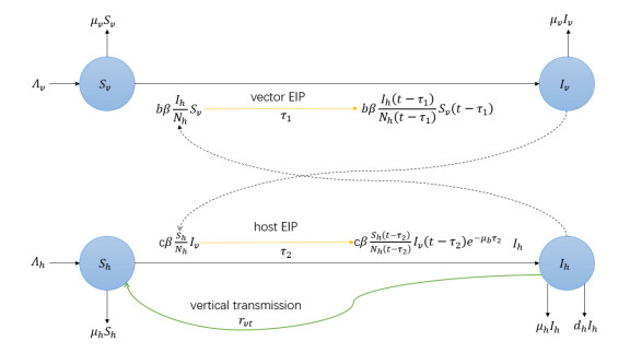
In this paper, we investigate a time-delayed vector-borne disease model with impulsive culling of the vector. The basic reproduction number $ \mathcal{R}_0 $ of our model is first introduced by the theory recently established in ^[1]. Then the threshold dynamics in terms of $ \mathcal{R}_0 $ are further developed. In particular, we show that if $ \mathcal{R}_0 < 1 $, then the disease will go extinct; if $ \mathcal{R}_0 > 1 $, then the disease will persist. The main mathematical approach is based on the uniform persistent theory for discrete-time semiflows on some appropriate Banach space. Finally, we carry out simulations to illustrate the analytic results and test the parametric sensitivity on $ \mathcal{R}_0 $.
- vector-borne,
- basic reproduction number,
- time delay,
- threshold dynamics,
- periodic culling
Citation: Rong Ming, Xiao Yu. Global dynamics of an impulsive vector-borne disease model with time delays[J]. Mathematical Biosciences and Engineering, 2023, 20(12): 20939-20958. doi: 10.3934/mbe.2023926

Related Papers:

Abstract

In this paper, we investigate a time-delayed vector-borne disease model with impulsive culling of the vector. The basic reproduction number $ \mathcal{R}_0 $ of our model is first introduced by the theory recently established in ^[1]. Then the threshold dynamics in terms of $ \mathcal{R}_0 $ are further developed. In particular, we show that if $ \mathcal{R}_0 < 1 $, then the disease will go extinct; if $ \mathcal{R}_0 > 1 $, then the disease will persist. The main mathematical approach is based on the uniform persistent theory for discrete-time semiflows on some appropriate Banach space. Finally, we carry out simulations to illustrate the analytic results and test the parametric sensitivity on $ \mathcal{R}_0 $.

References

[1]	Z. Bai, X. Q. Zhao, Basic reproduction ratios for periodic and time-delayed compartmental models with impulses, J. Math. Biol., 80 (2020), 1095–1117. https://doi.org/10.1007/s00285-019-01452-2 doi: 10.1007/s00285-019-01452-2
[2]	S. Ruan, D. Xiao, J. C. Beier, On the delayed Ross-Macdonald model for malaria transmission, Bull. Math. Biol., 70 (2008), 1098–1114. https://doi.org/10.1007/s11538-007-9292-z doi: 10.1007/s11538-007-9292-z
[3]	D. Nash, F. Mostashari, A. Fine, J. Miller, D. O'Leary, K. Murray, et al., The outbreak of West Nile virus infection in the New York City area in 1999, N. Engl. J. Med., 344 (2001), 1807–1814. https://doi.org/10.1056/NEJM200106143442401 doi: 10.1056/NEJM200106143442401
[4]	S. Tang, L. Chen, Density-dependent birth rate, birth pulses and their population dynamic consequences, J. Math. Biol., 44 (2002), 185–199. https://doi.org/10.1007/s002850100121 doi: 10.1007/s002850100121
[5]	Z. Bai, Y. Lou, X. Q. Zhao, A delayed succession model with diffusion for the impact of diapause on population growth, SIAM J. Appl. Math., 80 (2020), 1493–1519. https://doi.org/10.1137/19M1236448 doi: 10.1137/19M1236448
[6]	S. Gao, L. Chen, Z. Teng, Impulsive vaccination of an SEIRS model with time delay and varying total population size, Bull. Math. Biol., 69 (2007), 731–745. https://doi.org/10.1007/s11538-006-9149-x doi: 10.1007/s11538-006-9149-x
[7]	X. Meng, L. Chen, H. Cheng, Two profitless delays for the SEIRS epidemic disease model with nonlinear incidence and pulse vaccination, Appl. Math. Comput., 186 (2007), 516–529. https://doi.org/10.1016/j.amc.2006.07.124 doi: 10.1016/j.amc.2006.07.124
[8]	Y. P. Yang, Y. Xiao, Threshold dynamics for compartmental epidemic models with impulses, Nonlinear Anal. Real World Appl., 13 (2012), 224–234. https://doi.org/10.1016/j.nonrwa.2011.07.028 doi: 10.1016/j.nonrwa.2011.07.028
[9]	X. Xu, Y. Xiao, R. A. Cheke, Models of impulsive culling of vector to interrupt transmission of West Nile virus to host, Appl. Math. Model., 39 (2015), 3549–3568. https://doi.org/10.1016/j.apm.2014.10.072 doi: 10.1016/j.apm.2014.10.072
[10]	Z. Yang, C. Huang, X. Zou, Effect of impulsive controls in a model system for age-structured population over a patchy environment, J. Math. Biol., 76 (2018), 1387–1419. https://doi.org/10.1007/s00285-017-1172-z doi: 10.1007/s00285-017-1172-z
[11]	S. A. Gourley, R. Liu, J. Wu, Eradicating vector-borne diseases via age-structured culling, J. Math. Biol., 54 (2007), 309–335. https://doi.org/10.1007/s00285-006-0050-x doi: 10.1007/s00285-006-0050-x
[12]	A. J. Terry, Impulsive culling of a structured population on two patches. J. Math. Biol., 61 (2010), 843–875. https://doi.org/10.1007/s00285-009-0325-0 doi: 10.1007/s00285-009-0325-0
[13]	S. P. Rajasekar, M. Pitchaimani, Q. Zhu, Probing a stochastic epidemic hepatitis C virus model with a chronically infected treated population, Acta Math. Sci., 42 (2022), 2087–2112. https://doi.org/10.1007/s10473-022-0521-1 doi: 10.1007/s10473-022-0521-1
[14]	Y. Zhao, L. Wang, Practical exponential stability of impulsive stochastic food chain system with time-varying delays, Mathematics, 11 (2023), 147. https://doi.org/10.3390/math11010147 doi: 10.3390/math11010147
[15]	Y. Han, Z. Bai, Threshold dynamics of a West Nile virus model with impulsive culling and incubation period., Discrete Contin. Dyn. Syst. B, 27 (2022), 4515–4529. https://doi.org/10.3934/dcdsb.2021239 doi: 10.3934/dcdsb.2021239
[16]	Y. Lou, X. Q. Zhao, A theoretical approach to understanding population dynamics with seasonal developmental durations, J. Nonlinear Sci., 27 (2017), 573–603. https://doi.org/10.1007/s00332-016-9344-3 doi: 10.1007/s00332-016-9344-3
[17]	X. Wang, X. Q. Zhao, A periodic vector-bias malaria model with incubation period, SIAM J. Appl. Math., 77 (2017), 181–201. https://doi.org/10.1137/15M1046277 doi: 10.1137/15M1046277
[18]	F. B. Wang, R. Wu, X. Q. Zhao, A West Nile virus transmission model with periodic incubation periods, SIAM J. Appl. Dyn. Syst., 18 (2019), 1498–1535. https://doi.org/10.1137/18M123616 doi: 10.1137/18M123616
[19]	F. B. Wang, R. Wu, X. Yu, Threshold dynamics of a bat-borne rabies model with periodic incubation periods, Nonlinear Anal. Real World Appl., 61 (2021), 103340. https://doi.org/10.1016/j.nonrwa.2021.103340 doi: 10.1016/j.nonrwa.2021.103340
[20]	X. Liu, G. Ballinger, Continuous dependence on initial values for impulsive delay differential equations, Appl. Math. Lett., 17 (2004), 483–490. https://doi.org/10.1016/S0893-9659(04)90094-8 doi: 10.1016/S0893-9659(04)90094-8
[21]	X. Q. Zhao, Dynamical Systems in Population Biology, 2nd edition, CMS Books in Mathematics, Springer, 2017. https://doi.org/10.1007/978-3-319-56433-3
[22]	G. Ballinger, X. Liu, Existence, uniqueness and boundedness results for impulsive delay differential equations, Appl. Anal., 74 (2000), 71–93. https://doi.org/10.1080/00036810008840804 doi: 10.1080/00036810008840804
[23]	H. L. Smith, Monotone Dynamical Systems: An Introduction to the Theory of Competitive and Cooperative Systems, American Mathematical Society, Providence, RI, 1995. https://doi.org/10.1090/surv/041
[24]	D. Bainov, P. Simeonov, Impulsive Differential Equations: Periodic Solutions and Applications, Longman Harlow (1993), New York. https://doi.org/10.1201/9780203751206
[25]	X. Liang, X. Q. Zhao, Asymptotic speeds of spread and traveling waves for monotone semiflows with applications, Commun. Pure Appl. Math., 60 (2007), 1–40. https://doi.org/10.1002/cpa.20154 doi: 10.1002/cpa.20154
[26]	L. Burlando, Monotonicity of spectral radius for positive operators on ordered Banach spaces, Arch. Math., 56 (1991), 49–57. https://doi.org/10.1007/BF01190081 doi: 10.1007/BF01190081
[27]	T. Kato, Perturbation Theory for Linear Operators, Springer, 1976. https://doi.org/10.1007/978-3-642-66282-9
[28]	X. Liu, X. Shen, Y. Zhang, A comparison principle and stability for large-scale impulsive delay differential systems, ANZIAM J., 47 (2005), 203–235. https://doi.org/10.1017/S1446181100009998 doi: 10.1017/S1446181100009998
[29]	W. Hu, Q. Zhu, H. R. Karimi, Some improved Razumikhin stability criteria for impulsive stochastic delay differential systems, IEEE Trans. Autom. Control, 64 (2019), 5207–5213. https://doi.org/10.1109/TAC.2019.2911182 doi: 10.1109/TAC.2019.2911182
[30]	W. Hu, Q. Zhu, Stability criteria for impulsive stochastic functional differential systems with distributed delay dependent impulsive effects, IEEE Trans. Syst. Man Cybern. Syst., 51 (2021), 2027–2032. https://doi.org/10.1109/TSMC.2019.2905007 doi: 10.1109/TSMC.2019.2905007
[31]	M. Xia, L. Liu, J. Fang, Y. Zhang, Stability analysis for a class of stochastic differential equations with impulses, Mathematics, 11 (2023), 1541. https://doi.org/10.3390/math11061541 doi: 10.3390/math11061541

Reader Comments

Your name:*

Email:*
© 2023 the Author(s), licensee AIMS Press. This is an open access article distributed under the terms of the Creative Commons Attribution License (http://creativecommons.org/licenses/by/4.0)