Mathematical analysis and optimal control of an epidemic model with vaccination and different infectivity

Lili Liu; Xi Wang; Yazhi Li; Lili Liu; Xi Wang; Yazhi Li

doi:10.3934/mbe.2023925

Mathematical Biosciences and Engineering

2023, Volume 20, Issue 12: 20914-20938. doi: 10.3934/mbe.2023925

Previous Article Next Article

Research article

Mathematical analysis and optimal control of an epidemic model with vaccination and different infectivity

Lili Liu ¹,
Xi Wang ¹,
Yazhi Li ^{2
,
,}

1.
Shanxi Key Laboratory of Mathematical Techniques and Big Data Analysis on Disease Control and Prevention, Complex Systems Research Center, Shanxi University, Taiyuan 030006, China
2.
School of Mathematics and Statistics, Qiannan Normal University for Nationalities, Duyun 558000, China

Academic Editor: David M. Bortz

Received: 09 August 2023 Revised: 27 October 2023 Accepted: 31 October 2023 Published: 20 November 2023

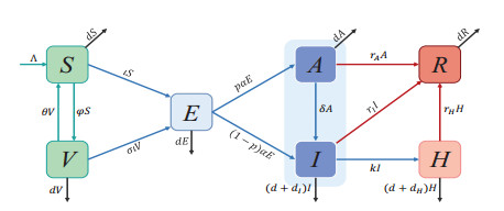
This paper aims to explore the complex dynamics and impact of vaccinations on controlling epidemic outbreaks. An epidemic transmission model which considers vaccinations and two different infection statuses with different infectivity is developed. In terms of a dynamic analysis, we calculate the basic reproduction number and control reproduction number and discuss the stability of the disease-free equilibrium. Additionally, a numerical simulation is performed to explore the effects of vaccination rate, immune waning rate and vaccine ineffective rate on the epidemic transmission. Finally, a sensitivity analysis revealed three factors that can influence the threshold: transmission rate, vaccination rate, and the hospitalized rate. In terms of optimal control, the following three time-related control variables are introduced to reconstruct the corresponding control problem: reducing social distance, enhancing vaccination rates, and enhancing the hospitalized rates. Moreover, the characteristic expression of optimal control problem. Four different control combinations are designed, and comparative studies on control effectiveness and cost effectiveness are conducted by numerical simulations. The results showed that Strategy C (including all the three controls) is the most effective strategy to reduce the number of symptomatic infections and Strategy A (including reducing social distance and enhancing vaccination rate) is the most cost-effective among the three strategies.
- epidemic model,
- vaccination,
- different infectivity,
- optimal control,
- cost-effectiveness
Citation: Lili Liu, Xi Wang, Yazhi Li. Mathematical analysis and optimal control of an epidemic model with vaccination and different infectivity[J]. Mathematical Biosciences and Engineering, 2023, 20(12): 20914-20938. doi: 10.3934/mbe.2023925

Related Papers:

Abstract

This paper aims to explore the complex dynamics and impact of vaccinations on controlling epidemic outbreaks. An epidemic transmission model which considers vaccinations and two different infection statuses with different infectivity is developed. In terms of a dynamic analysis, we calculate the basic reproduction number and control reproduction number and discuss the stability of the disease-free equilibrium. Additionally, a numerical simulation is performed to explore the effects of vaccination rate, immune waning rate and vaccine ineffective rate on the epidemic transmission. Finally, a sensitivity analysis revealed three factors that can influence the threshold: transmission rate, vaccination rate, and the hospitalized rate. In terms of optimal control, the following three time-related control variables are introduced to reconstruct the corresponding control problem: reducing social distance, enhancing vaccination rates, and enhancing the hospitalized rates. Moreover, the characteristic expression of optimal control problem. Four different control combinations are designed, and comparative studies on control effectiveness and cost effectiveness are conducted by numerical simulations. The results showed that Strategy C (including all the three controls) is the most effective strategy to reduce the number of symptomatic infections and Strategy A (including reducing social distance and enhancing vaccination rate) is the most cost-effective among the three strategies.

References

[1]	J. T. Wu, K. Leung, G. M. Leung, Nowcasting and forecasting the potential domestic and international spread of the 2019-nCoV outbreak originating in Wuhan, China: a modelling study, Lancet, 395 (2020), 689–697. https://doi.org/10.1016/S0140-6736(20)30260-9 doi: 10.1016/S0140-6736(20)30260-9
[2]	K. M. Bubar, K. Reinholt, S. M. Kissler, M. Lipsitch, S. Cobey, Y. H. Grad, et al., Model-informed COVID-19 vaccine prioritization strategies by age and serostatus, Science, 371 (2021), 916–921. https://doi.org/10.1126/science.abe6959 doi: 10.1126/science.abe6959
[3]	E. A. Iboi, C. N. Ngonghala, A. B. Gumel, Will an imperfect vaccine curtail the COVID-19 pandemic in the US?, Infect. Dis. Model., 5 (2020), 510–524. https://doi.org/10.1016/j.idm.2020.07.006 doi: 10.1016/j.idm.2020.07.006
[4]	Z. Chen, K. Liu, X. Liu, Y. Lou, Modelling epidemics with fractional-dose vaccination in response to limited vaccine supply, J. Theor. Biol., 486 (2020), 110085. https://doi.org/10.1016/j.jtbi.2019.110085 doi: 10.1016/j.jtbi.2019.110085
[5]	S. Gao, M. Martcheva, H. Miao, L. Rong, A two-sex model of human papillomavirus infection: Vaccination strategies and a case study, J. Theor. Biol., 536 (2022), 111006. https://doi.org/10.1016/j.jtbi.2022.111006 doi: 10.1016/j.jtbi.2022.111006
[6]	J. Thompson, S. Wattam, Estimating the impact of interventions against covid-19: From lockdown to vaccination, PLoS One, 16 (2021), e0261330. https://doi.org/10.1371/journal.pone.0261330 doi: 10.1371/journal.pone.0261330
[7]	I. Harizi, S. Berkane, A. Tayebi, Modeling the effect of population-wide vaccination on the evolution of COVID-19 epidemic in Canada, medRxiv, (2021), 2021–02. https://doi.org/10.1101/2021.02.05.21250572
[8]	M. Diagne, H. Rwezaura, S. Tchoumi, J. Tchuenche, Comput. Math. Methods Med., 2021 (2021). https://doi.org/10.1155/2021/1250129
[9]	J. N. Paul, I. S. Mbalawata, S. S. Mirau, L. Masandawa, Mathematical modeling of vaccination as a control measure of stress to fight COVID-19 infections, Chaos, Solitons Fractals, 166 (2023), 112920. https://doi.org/10.1016/j.chaos.2022.112920 doi: 10.1016/j.chaos.2022.112920
[10]	C. R. Xavier, R. S. Oliveira, V. da Fonseca Vieira, B. M. Rocha, R. F. Reis, B. de Melo Quintela, et al., Timing the race of vaccination, new variants, and relaxing restrictions during COVID-19 pandemic, J. Comput. Sci., 61 (2022), 101660. https://doi.org/10.1016/j.jocs.2022.101660 doi: 10.1016/j.jocs.2022.101660
[11]	M. Makhoul, H. Chemaitelly, H. H. Ayoub, S. Seedat, L. J. Abu-Raddad, Epidemiological differences in the impact of COVID-19 vaccination in the United States and China, Vaccines, 9 (2021), 223. https://doi.org/10.3390/vaccines9030223 doi: 10.3390/vaccines9030223
[12]	M. Makhoul, H. H. Ayoub, H. Chemaitelly, S. Seedat, G. R. Mumtaz, S. Al-Omari, et al., Epidemiological impact of SARS-CoV-2 vaccination: Mathematical modeling analyses, Vaccines, 8 (2020), 668. https://doi.org/10.3390/vaccines8040668 doi: 10.3390/vaccines8040668
[13]	A. Olivares, E. Staffetti, Uncertainty quantification of a mathematical model of COVID-19 transmission dynamics with mass vaccination strategy, Chaos, Solitons Fractals, 146 (2021), 110895. https://doi.org/10.1016/j.chaos.2021.110895 doi: 10.1016/j.chaos.2021.110895
[14]	B. H. Foy, B. Wahl, K. Mehta, A. Shet, G. I. Menon, C. Britto, Comparing COVID-19 vaccine allocation strategies in India: A mathematical modelling study, Infect. Dis. Model., 103 (2021), 431–438. https://doi.org/10.1016/j.ijid.2020.12.075 doi: 10.1016/j.ijid.2020.12.075
[15]	R. Li, H. Liu, C. K. Fairley, Z. Zou, L. Xie, X. Li, et al., Cost-effectiveness analysis of BNT162b2 COVID-19 booster vaccination in the United States, Infect. Dis. Model., 119 (2022), 87–94. https://doi.org/10.1016/j.ijid.2022.03.029 doi: 10.1016/j.ijid.2022.03.029
[16]	H. Alrabaiah, M. A. Safi, M. H. DarAssi, B. Al-Hdaibat, S. Ullah, M. A. Khan, et al., Optimal control analysis of hepatitis B virus with treatment and vaccination, Results Phys., 19 (2020), 103599. https://doi.org/10.1016/j.rinp.2020.103599 doi: 10.1016/j.rinp.2020.103599
[17]	U. Odionyenma, A. Omame, N. Ukanwoke, I. Nometa, Optimal control of Chlamydia model with vaccination, Int. J. Dyn. Control, 10 (2022), 332–348. https://doi.org/10.1016/j.rinp.2020.103599 doi: 10.1016/j.rinp.2020.103599
[18]	M. Mandal, S. Jana, S. K. Nandi, A. Khatua, S. Adak, T. Kar, A model based study on the dynamics of COVID-19: Prediction and control, Chaos, Solitons Fractals, 136 (2020), 109889. https://doi.org/10.1016/j.chaos.2020.109889. doi: 10.1016/j.chaos.2020.109889
[19]	M. A. Khan, A. Atangana, Mathematical modeling and analysis of COVID-19: A study of new variant Omicron, Physica A, 599 (2022), 127452. https://doi.org/10.1016/j.physa.2022.127452 doi: 10.1016/j.physa.2022.127452
[20]	Y. Choi, J. S. Kim, J. E. Kim, H. Choi, C. H. Lee, Vaccination prioritization strategies for COVID-19 in Korea: a mathematical modeling approach, Int. J. Public Health, 18 (2021), 4240. https://doi.org/10.3390/ijerph18084240 doi: 10.3390/ijerph18084240
[21]	P. Samui, J. Mondal, S. Khajanchi, A mathematical model for COVID-19 transmission dynamics with a case study of India, Chaos, Solitons Fractals, 140 (2020), 110173. https://doi.org/10.1016/j.chaos.2020.110173 doi: 10.1016/j.chaos.2020.110173
[22]	A. A. Khan, S. Ullah, R. Amin, Optimal control analysis of COVID-19 vaccine epidemic model: a case study, Eur. Phys. J. Plus, 137 (2022), 1–25. https://doi.org/10.1140/epjp/s13360-022-02365-8 doi: 10.1140/epjp/s13360-022-02365-8
[23]	Q. Li, B. Tang, N. L. Bragazzi, Y. Xiao, J. Wu, Modeling the impact of mass influenza vaccination and public health interventions on COVID-19 epidemics with limited detection capability, Math. Biosci., 325 (2020), 108378. https://doi.org/10.1016/j.mbs.2020.108378 doi: 10.1016/j.mbs.2020.108378
[24]	W. Zhou, B. Tang, Y. Bai, Y. Shao, Y. Xiao, S. Tang, The resurgence risk of COVID-19 in the presence of immunity waning and ADE effect: a mathematical modelling study, Vaccines, 40 (2022), 7147–7150. https://doi.org/10.1101/2021.08.25.21262601 doi: 10.1101/2021.08.25.21262601
[25]	E. Alzahrani, M. El-Dessoky, D. Baleanu, Mathematical modeling and analysis of the novel Coronavirus using Atangana–Baleanu derivative, Results Phys., 25 (2021), 104240. https://doi.org/10.1016/j.rinp.2021.104240 doi: 10.1016/j.rinp.2021.104240
[26]	B. Buonomo, R. Della Marca, A. d'Onofrio, M. Groppi, A behavioural modelling approach to assess the impact of COVID-19 vaccine hesitancy, J. Theor. Biol., 534 (2022), 110973. https://doi.org/10.1016/j.jtbi.2021.110973 doi: 10.1016/j.jtbi.2021.110973
[27]	S. Bugalia, V. P. Bajiya, J. P. Tripathi, M. T. Li, G. Q. Sun, Mathematical modeling of COVID-19 transmission: the roles of intervention strategies and lockdown, Math. Biosci. Eng., 17 (2020), 5961–5986. https://doi.org/10.3934/mbe.2020318 doi: 10.3934/mbe.2020318
[28]	F. Ndaïrou, I. Area, J. J. Nieto, D. F. Torres, Mathematical modeling of COVID-19 transmission dynamics with a case study of Wuhan, Chaos, Solitons Fractals, 135 (2020), 109846. https://doi.org/10.1016/j.chaos.2020.109846 doi: 10.1016/j.chaos.2020.109846
[29]	D. Aldila, B. M. Samiadji, G. M. Simorangkir, S. H. Khosnaw, M. Shahzad, Impact of early detection and vaccination strategy in COVID-19 eradication program in Jakarta, Indonesia, BMC Res. Notes, 14 (2021), 1–7. https://doi.org/10.1186/s13104-021-05540-9 doi: 10.1186/s13104-021-05540-9
[30]	P. Dreessche, J. Watmough, Reproduction numbers and sub-threshold endemic equilibria for compartmental models of disease transmission, Math. Biosci., 180 (2002), 29–48. https://doi.org/10.1016/S0025-5564(02)00108-6 doi: 10.1016/S0025-5564(02)00108-6
[31]	O. Diekmann, J. A. P. Heesterbeek, J. A. Metz, On the definition and the computation of the basic reproduction ratio ${R}_ 0$ in models for infectious diseases in heterogeneous populations, J. Math. Biol., 28 (1990), 365–382. https://doi.org/10.1007/BF00178324 doi: 10.1007/BF00178324
[32]	C. Xu, G. Gertner, Extending a global sensitivity analysis technique to models with correlated parameters, Comput. Stat. Data Anal., 51 (2007), 5579–5590. https://doi.org/10.1016/j.csda.2007.04.003 doi: 10.1016/j.csda.2007.04.003
[33]	Z. Zi, Sensitivity analysis approaches applied to systems biology models, IET Syst. Biol., 5 (2011), 336–346. https://doi.org/10.1049/iet-syb.2011.0015 doi: 10.1049/iet-syb.2011.0015
[34]	A. K. Paul, M. A. Kuddus, Mathematical analysis of a COVID-19 model with double dose vaccination in Bangladesh, Results Phys., 35 (2022), 105392. https://doi.org/10.1016/j.rinp.2022.105392 doi: 10.1016/j.rinp.2022.105392
[35]	S. M. Blower, H. Dowlatabadi, Sensitivity and uncertainty analysis of complex models of disease transmission: an HIV model, as an example, Int. Stat. Rev., 62 (1994), 229–243. https://doi.org/10.2307/1403510 doi: 10.2307/1403510
[36]	S. Marino, I. B. Hogue, C. J. Ray, D. E. Kirschner, A methodology for performing global uncertainty and sensitivity analysis in systems biology, J. Theor. Biol., 254 (2008), 178–196. https://doi.org/10.1016/j.jtbi.2008.04.011 doi: 10.1016/j.jtbi.2008.04.011
[37]	D. L. Lukes, Differential Equations: Classical to Controlled, New York: Academic press, 1982.
[38]	L. S. Pontryagin, Mathematical Theory of Optimal Processes, Florida: CRC press, 1987.
[39]	Z. H. Shen, Y. M. Chu, M. A. Khan, S. Muhammad, O. A. Al-Hartomy, M. Higazy, Mathematical modeling and optimal control of the COVID-19 dynamics, Results Phys., 31 (2021), 105028. https://doi.org/10.1016/j.rinp.2021.105028 doi: 10.1016/j.rinp.2021.105028
[40]	S. Lenhart, J. T. Workman, Optimal Control Applied to Biological Models, Boca Raton: Chapman and Hall/CRC, 2007.
[41]	K. O. Okosun, O. Rachid, N. Marcus, Optimal control strategies and cost-effectiveness analysis of a malaria model, BioSystems, 111 (2013), 83–101. https://doi.org/10.1016/j.biosystems.2012.09.008 doi: 10.1016/j.biosystems.2012.09.008
[42]	J. K. K. Asamoah, E. Okyere, A. Abidemi, S. E. Moore, G. Q. Sun, Z. Jin, et al., Optimal control and comprehensive cost-effectiveness analysis for COVID-19, Results Phys., 33 (2022), 105177. https://doi.org/10.1016/j.rinp.2022.105177 doi: 10.1016/j.rinp.2022.105177
[43]	Y. Tao, S. A. Campbell, F. J. Poulin, Dynamics of a diffusive nutrient-phytoplankton-zooplankton model with spatio-temporal delay, SIAM J. Appl. Math., 81 (2021), 2405–2432. https://doi.org/10.1137/20M1378065 doi: 10.1137/20M1378065
[44]	T Jiang, Q, Jin, J. Wang, F. Wu, J. Chen, G. Chen, et al. HLA-I evolutionary divergence confers response to PD-1 blockade plus chemotherapy in untreated advanced non-small cell Lung cancer, Clin. Cancer Res., 2023 (2023), OF1–OF14. https://doi.org/10.1158/1078-0432.CCR-23-0604 doi: 10.1158/1078-0432.CCR-23-0604
[45]	Y. Tao, Y. Sun, H. Zhu, J. Lyu, J. Ren, Nilpotent singularities and periodic perturbation of a $GI\beta$ model: A pathway to Glucose disorder, J. Nonlinear Sci., 33 (2023), 49. https://doi.org/10.1007/s00332-023-09907-z doi: 10.1007/s00332-023-09907-z
[46]	B. Yang, Z. Yu, Y. Cai, The impact of vaccination on the spread of COVID-19: Studying by a mathematical model, Physica A, 590 (2022), 126717. https://doi.org/10.1016/j.physa.2021.126717 doi: 10.1016/j.physa.2021.126717

Reader Comments

Your name:*

Email:*
© 2023 the Author(s), licensee AIMS Press. This is an open access article distributed under the terms of the Creative Commons Attribution License (http://creativecommons.org/licenses/by/4.0)