As an essential component of mechanical equipment, the fault diagnosis of rolling bearings may not only guarantee the systematic operation of the equipment, but also minimize any financial losses caused by equipment shutdowns. Fault diagnosis algorithms based on convolutional neural networks (CNN) have been widely used. However, traditional CNNs have limited feature representation capabilities, thereby making it challenging to determine their hyperparameters. This paper proposes a fault diagnosis method that combines a 1D-CNN with an attention mechanism and hyperparameter optimization to overcome the aforementioned limitations; this method improves the search speed for optimal hyperparameters of CNN models, improves the diagnostic accuracy, and enhances the representation of fault feature information in CNNs. First, the 1D-CNN is improved by combining it with an attention mechanism to enhance the fault feature information. Second, a swarm intelligence algorithm based on Differential Evolution (DE) and Grey Wolf Optimization (GWO) is proposed, which not only improves the convergence accuracy, but also increases the search efficiency. Finally, the improved 1D-CNN alongside hyperparameters optimization are used to diagnose the faults of rolling bearings. By using the Case Western Reserve University (CWRU) and Jiangnan University (JNU) datasets, when compared to other common diagnosis models, the results demonstrate the usefulness and dependability of the DE-GWO-CNN algorithm in fault diagnosis applications by demonstrating the increased diagnostic accuracy and superior anti-noise capabilities of the proposed method. The fault diagnosis methodology presented in this paper can accurately identify faults and provide dependable fault classification, thereby assisting technicians in promptly resolving faults and minimizing equipment failures and operational instabilities.
Citation: Qiushi Wang, Zhicheng Sun, Yueming Zhu, Chunhe Song, Dong Li. Intelligent fault diagnosis algorithm of rolling bearing based on optimization algorithm fusion convolutional neural network[J]. Mathematical Biosciences and Engineering, 2023, 20(11): 19963-19982. doi: 10.3934/mbe.2023884
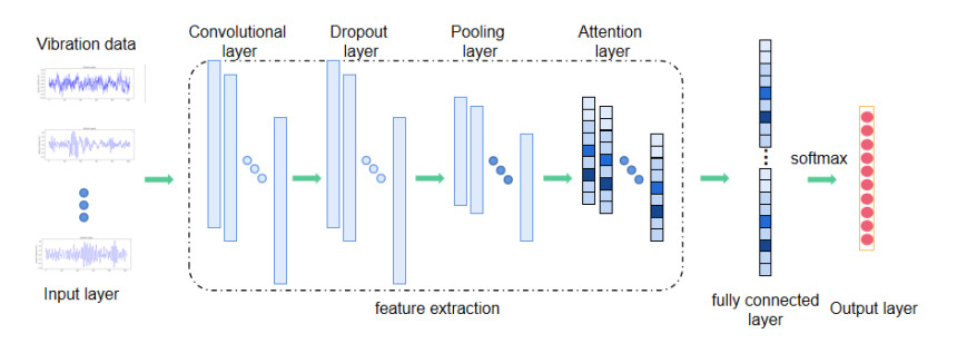
As an essential component of mechanical equipment, the fault diagnosis of rolling bearings may not only guarantee the systematic operation of the equipment, but also minimize any financial losses caused by equipment shutdowns. Fault diagnosis algorithms based on convolutional neural networks (CNN) have been widely used. However, traditional CNNs have limited feature representation capabilities, thereby making it challenging to determine their hyperparameters. This paper proposes a fault diagnosis method that combines a 1D-CNN with an attention mechanism and hyperparameter optimization to overcome the aforementioned limitations; this method improves the search speed for optimal hyperparameters of CNN models, improves the diagnostic accuracy, and enhances the representation of fault feature information in CNNs. First, the 1D-CNN is improved by combining it with an attention mechanism to enhance the fault feature information. Second, a swarm intelligence algorithm based on Differential Evolution (DE) and Grey Wolf Optimization (GWO) is proposed, which not only improves the convergence accuracy, but also increases the search efficiency. Finally, the improved 1D-CNN alongside hyperparameters optimization are used to diagnose the faults of rolling bearings. By using the Case Western Reserve University (CWRU) and Jiangnan University (JNU) datasets, when compared to other common diagnosis models, the results demonstrate the usefulness and dependability of the DE-GWO-CNN algorithm in fault diagnosis applications by demonstrating the increased diagnostic accuracy and superior anti-noise capabilities of the proposed method. The fault diagnosis methodology presented in this paper can accurately identify faults and provide dependable fault classification, thereby assisting technicians in promptly resolving faults and minimizing equipment failures and operational instabilities.

| [1] |
C. Liu, X. Zhang, Z. Bao, Z. He, M. Gao, W. Song, A novel deep transfer learning method for intelligent fault diagnosis based on variational mode decomposition and efficient channel attention, Entropy, 24 (2022), 1087. https://doi.org/10.3390/e24081087 doi: 10.3390/e24081087

|
| [2] |
Z. Hou, J. Zeng, Condition monitoring technology for bearing ring groove grinding, J. Phys. Conf. Ser., 1213 (2019), 052036. https://doi.org/10.1088/1742-6596/1213/5/052036 doi: 10.1088/1742-6596/1213/5/052036
|
| [3] |
X. Gao, H. Wei, T. Li, G. Yang, A rolling bearing fault diagnosis method based on LSSVM, Adv. Mechan. Eng., 12 (2020), 1–10. https://doi.org/10.1177/1687814019899561 doi: 10.1177/1687814019899561
|
| [4] |
Z. Yan, G. Liu, J. Wang, H. Bao, Z. Zhang, X. Zhang, et al., A new universal domain adaptive method for diagnosing unknown bearing faults, Entropy, 23 (2021), 1052. https://doi.org/10.3390/e23081052 doi: 10.3390/e23081052
|
| [5] |
J. Tang, J. Hu, J. Qing, T. Kang, Rolling bearing fault monitoring for sparse time-frequency representation and feature detection strategy, Entropy, 24 (2022), 1822. https://doi.org/10.3390/e24121822 doi: 10.3390/e24121822
|
| [6] |
Y. Zhang, L. Duan, M. L. Duan, A new feature extraction approach using improved symbolic aggregate approximation for machinery intelligent diagnosis, Measurement, 133 (2019), 468–478. https://doi.org/10.1016/j.measurement.2018.10.045 doi: 10.1016/j.measurement.2018.10.045
|
| [7] |
Z. Wang, X. He, B. Yang, N. Li, Subdomain adaptation transfer learning network for fault diagnosis of roller bearings, IEEE Trans. Ind. Electron., 69 (2022), 8430–8439. https://doi.org/10.1109/TIE.2021.3108726 doi: 10.1109/TIE.2021.3108726
|
| [8] |
W. Li, Y. Cao, L. Li, S. Hou, An orthogonal wavelet transform-based k-nearest neighbor algorithm to detect faults in bearings, Shock Vibr., 2022 (2022), 1–13. https://doi.org/10.1155/2022/5242106 doi: 10.1155/2022/5242106
|
| [9] |
D. Wu, C. Jemmings, J. Terpenn, A comparative study on machine learning algorithms for smart manufacturing: tool wear prediction using random forests, J. Manuf. Sci. Eng. Trans. ASME, 139 (2017), 179–187. https://doi.org/10.1115/1.4036350 doi: 10.1115/1.4036350
|
| [10] |
S. Guo, B. Zhang, T. Yang, D. Lyu, W. Gao, Multitask convolutional neural network with information fusion for bearing fault diagnosis and localization, IEEE Transact. Industr. Electron., 67 (2020), 8005–8015. https://doi.org/10.1109/TIE.2019.2942548 doi: 10.1109/TIE.2019.2942548
|
| [11] |
H. Pan, X. He, S. Tang, F. Meng, An improved bearing fault diagnosis method using one-dimensional CNN and LSTM, J. Mechan. Eng., 64 (2018), 443–452. https://doi.org/10.5545/sv-jme.2018.5249 doi: 10.5545/sv-jme.2018.5249
|
| [12] |
Z. Meng, W. Cao, D. Sun, Q. Li, W. Ma, F. Fan. Research on fault diagnosis method of MS-CNN rolling bearing based on local central moment discrepancy, Adv. Eng. Inform., 54 (2022), 101797. https://doi.org/10.1016/j.aei.2022.101797 doi: 10.1016/j.aei.2022.101797
|
| [13] |
W. Deng, H. Liu, J. Xu, H. Zhao, Y. Song, An improved quantum-inspired differential evolution algorithm for deep belief network, IEEE Transact. Instrument. Measur., 69 (2020), 7319–7327. https://doi.org/10.1109/TIM.2020.2983233 doi: 10.1109/TIM.2020.2983233
|
| [14] |
J. Yuan, R. Zhao, T. He, P. Chen, K. Wei, Z. Xing, Fault diagnosis of rotor based on Semi-supervised Multi-Graph Joint Embedding, ISA Trans., 131 (2022), 516–532, https://doi.org/10.1016/j.isatra.2022.05.006 doi: 10.1016/j.isatra.2022.05.006
|
| [15] |
Q. Ni, J.C. Ji, H. Benjamin, K. Feng, K. A. Nandi, Physics-Informed Residual Network (PIResNet) for rolling element bearing fault diagnostics, Mechan. Syst. Signal Process., 200 (2023), 110544. https://doi.org/10.1016/j.ymssp.2023.110544 doi: 10.1016/j.ymssp.2023.110544
|
| [16] |
K. Feng, J. C. Ji, Y. Zhang, Q. Ni, Z. Liu, B. Michael, Digital twin-driven intelligent assessment of gear surface degradation, Mechan. Syst. Signal Process., 186 (2023), 109896. https://doi.org/10.1016/j.ymssp.2022.109896 doi: 10.1016/j.ymssp.2022.109896
|
| [17] |
J. Yuan, R. Zhao, P. Chen, T. He, K. Wei, Dimensionality reduction using local-global standard hypergraph embedding for rotor fault diagnosis, Meas. Sci. Technol., 34 (2023), 034006. https://doi.org/10.1088/1361-6501/acab1e doi: 10.1088/1361-6501/acab1e
|
| [18] |
P. Wang, R. Yan, R. Gao, Virtualization and deep recognition for system fault classification, J. Manuf. Syst., 44 (2017), 310–316. https://doi.org/10.1016/j.jmsy.2017.04.012 doi: 10.1016/j.jmsy.2017.04.012
|
| [19] |
J. Qiu, H. Tao, L. Cheng, L. Shen, Bearing fault diagnosis based on self-attention mechanism ACGAN, Inform. Control., 51 (2022), 753–762. https://doi.org/10.13976/j.cnki.xk.2022.2002 doi: 10.13976/j.cnki.xk.2022.2002
|
| [20] |
S. Gao, S. Shi, Y. Zhang, Rolling bearing compound fault diagnosis based on parameter optimization MCKD and convolutional neural network, IEEE Trans. Instrum. Meas., 71 (2022), 1–8. https://doi.org/10.1109/TIM.2022.3158379 doi: 10.1109/TIM.2022.3158379
|
| [21] |
D. Hoang, H. Kang, Rolling element bearing fault diagnosis using convolutional neural network and vibration image, Cogn. Syst. Res., 53 (2018), 42–50. https://doi.org/10.1016/j.cogsys.2018.03.002 doi: 10.1016/j.cogsys.2018.03.002
|
| [22] |
M. Wang, W. Wang, X. Zhang, Iu HH-C, A new fault diagnosis of rolling bearing based on markov transition field and CNN, Entropy, 24 (2022), 751. https://doi.org/10.3390/e24060751 doi: 10.3390/e24060751
|
| [23] |
X. Zhao, K. Ji, M. Zhang, H. Huang, F. Wang, Y. Liu, et al., Intelligent fault diagnosis of gearbox under variable working conditions with adaptive intraclass and interclass convolutional neural network, IEEE Transact. Neural Networks Learn. Syst., 34 (2023), 6339–6353. https://doi.org/10.1109/TNNLS.2021.3135877 doi: 10.1109/TNNLS.2021.3135877
|
| [24] |
W. Deng, X. Zhang, Y. Zhou, Y. Liu, X. Zhou, H. Chen, et al., An enhanced fast non-dominated solution sorting genetic algorithm for multi-objective problems, Inform. Sci., 585 (2022), 441–453. https://doi.org/10.1016/j.ins.2021.11.052 doi: 10.1016/j.ins.2021.11.052
|
| [25] |
Q. Sun, Y. Li, Research on fault diagnosis of rolling bearings based on de algorithm optimization of CNN, Noise Vibr. Control, 42 (2022), 165–171. https://doi.org/10.3969/j.issn.1006-1355.2022.04.027 doi: 10.3969/j.issn.1006-1355.2022.04.027
|
| [26] |
Y. Li, J. Ma, L. Jiang, Fault diagnosis of rolling bearing based on an improved convolutional neural network using SFLA, J. Vibr. Shock, 39 (2020), 187–193. https://doi.org/10.13465/j.cnki.jvs.2020.24.026 doi: 10.13465/j.cnki.jvs.2020.24.026
|
| [27] |
X. Wang, X. Liu, J. Wang, X. Xiong, S. Bi, Z. Deng, Improved variational mode decomposition and one-dimensional CNN network with parametric rectified linear unit (PReLU) approach for rolling bearing fault diagnosis, Appl. Sci., 12 (2022), 9324. https://doi.org/10.3390/app12189324 doi: 10.3390/app12189324
|
| [28] |
G. Ning, D. Cao, Y. Zhou, Improved differential evolution algorithm for solving 0-1 programming problems, J. Syst. Sci. Math. Sci., 39 (2019), 120–132. https://doi.org/10.12341/jssms13549 doi: 10.12341/jssms13549
|
| [29] |
X. Zhang, X. Wang, Comprehensive review of grey wolf optimization algorithm, Computer Sci., 46 (2019), 30–38. https://doi.org/10.11896/j.issn.1002-137X.2019.03.004 doi: 10.11896/j.issn.1002-137X.2019.03.004
|
| [30] |
J. Jiao, M. Zhao, J. Lin, K. Liang, A comprehensive review on convolutional neural network in machine fault diagnosis, Neuro. Comput., 471 (2020), 36–63. https://doi.org/10.1016/j.neucom.2020.07.088 doi: 10.1016/j.neucom.2020.07.088
|
| [31] |
G. Brauwers, F. Frasincar, A general survey on attention mechanisms in deep learning, IEEE Transact. Knowl. Data Eng., 35 (2023), 3279–3298. https://doi.org/10.1109/TKDE.2021.3126456 doi: 10.1109/TKDE.2021.3126456
|
| [32] |
N. Nahak, R. K. Mallick, Damping of power system oscillations by a novel DE-GWO optimized dual UPFC controller, Eng. Sci. Technol. Int. J., 20 (2017), 1275–1284. https://doi.org/10.1016/j.jestch.2017.09.001 doi: 10.1016/j.jestch.2017.09.001
|
| [33] |
M. Yu, D. Wang, Model-based health monitoring for a vehicle steering system with multiple faults of unknown types, IEEE Transact. Industr. Electron., 61 (2014), 3574–3586. https://doi.org/10.1109/TIE.2013.2281159 doi: 10.1109/TIE.2013.2281159
|
| [34] |
Z. Jin, D. He, Z. Wei, Intelligent fault diagnosis of train axle box bearing based on parameter optimization VMD and improved DBN, Eng. Appl. Artif. Intell., 110 (2022), 104713. https://doi.org/10.1016/j.engappai.2022.104713 doi: 10.1016/j.engappai.2022.104713
|
| [35] |
K. Li, X. Ping, H. Wang, P. Chen, Y. Cao, Sequential fuzzy diagnosis method for motor roller bearing in variable operating conditions based on vibration analysis, Sensors, 13 (2013), 8013–8041. https://doi.org/10.3390/s130608013 doi: 10.3390/s130608013
|
| [36] |
Q. Gu, X. Li, C. Lu, Hybrid genetic greywolf algorithm for high dimensional complex function optimization, Control Decision, 35 (2020), 1191–1198. https://doi.org/10.13195/j.kzyjc.2018.1253 doi: 10.13195/j.kzyjc.2018.1253
|
| [37] |
Z. Teng, J. Lv, L. Guo, An improved hybrid greywolf optimization algorithm, Soft Computing, 23 (2019), 6617–6631. https://doi.org/10.1007/s00500-018-3310-y doi: 10.1007/s00500-018-3310-y
|
| [38] |
R. Sun, J. Yang, D. Yao, J. Wang, A new method of wheelset bearing fault diagnosis, Entropy, 24 (2022), 1381. https://doi.org/10.3390/e24101381 doi: 10.3390/e24101381
|


Figures(11) / Tables(10)

Qiushi Wang, Zhicheng Sun, Yueming Zhu, Chunhe Song, Dong Li. Intelligent fault diagnosis algorithm of rolling bearing based on optimization algorithm fusion convolutional neural network[J]. Mathematical Biosciences and Engineering, 2023, 20(11): 19963-19982. doi: 10.3934/mbe.2023884


 DownLoad: