Entropy-based reliable non-invasive detection of coronary microvascular dysfunction using machine learning algorithm

Xiaoye Zhao; Yinlan Gong; Lihua Xu; Ling Xia; Jucheng Zhang; Dingchang Zheng; Zongbi Yao; Xinjie Zhang; Haicheng Wei; Jun Jiang; Haipeng Liu; Jiandong Mao; Xiaoye Zhao; Yinlan Gong; Lihua Xu; Ling Xia; Jucheng Zhang; Dingchang Zheng; Zongbi Yao; Xinjie Zhang; Haicheng Wei; Jun Jiang; Haipeng Liu; Jiandong Mao

doi:10.3934/mbe.2023582

Mathematical Biosciences and Engineering

2023, Volume 20, Issue 7: 13061-13085. doi: 10.3934/mbe.2023582

Previous Article Next Article

Research article Special Issues

Entropy-based reliable non-invasive detection of coronary microvascular dysfunction using machine learning algorithm

1.
School of Instrument Science and Opto-electronic Engineering, Hefei University of Technology, Hefei 230009, Anhui, China
2.
School of Electrical and Information Engineering, North Minzu University, Yinchuan 750001, Ningxia, China
3.
Key Laboratory of Atmospheric Environment Remote Sensing of Ningxia, Yinchuan 750001, Ningxia, China
4.
Institute of Wenzhou, Zhejiang University, Wenzhou 325000, Zhejiang, China
5.
Hangzhou Linghua Biotech Ltd, Hangzhou 310009, Zhejiang, China
6.
Key Laboratory for Biomedical Engineering of Ministry of Education, Hangzhou 310009, Zhejiang, China
7.
Institute of Biomedical Engineering, Zhejiang University, Hangzhou 310009, Zhejiang, China
8.
Department of Clinical Engineering, The Second Affiliated Hospital, Zhejiang University School of Medicine, Hangzhou 310009, Zhejiang, China
9.
Research Centre for Intelligent Healthcare, Coventry University, Coventry, CV1 5FB, United Kingdom
10.
Department of Cardiology, Ningxia Hui Autonomous Region People's Hospital, Yinchuan 750021, Ningxia, China
11.
Department of Cardiology, The Second Affiliated Hospital, Zhejiang University School of Medicine, Hangzhou 310009, Zhejiang, China

Academic Editor: Ulf Schmitz
† These two authors contributed equally.

Received: 29 January 2023 Revised: 20 May 2023 Accepted: 22 May 2023 Published: 05 June 2023

Purpose
Coronary microvascular dysfunction (CMD) is emerging as an important cause of myocardial ischemia, but there is a lack of a non-invasive method for reliable early detection of CMD.

Aim
To develop an electrocardiogram (ECG)-based machine learning algorithm for CMD detection that will lay the groundwork for patient-specific non-invasive early detection of CMD.

Methods
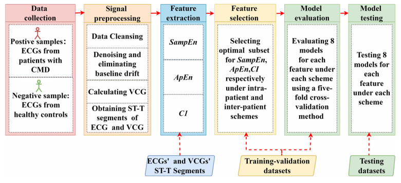
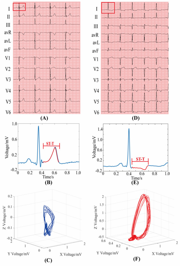
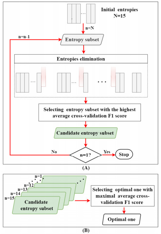
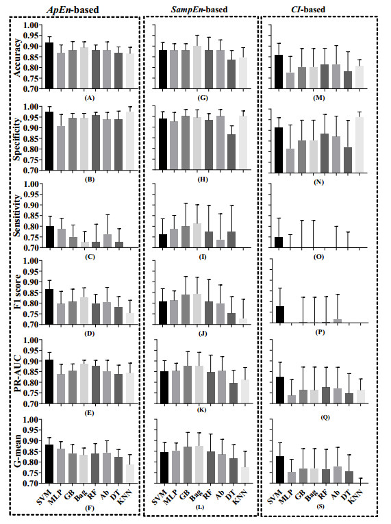
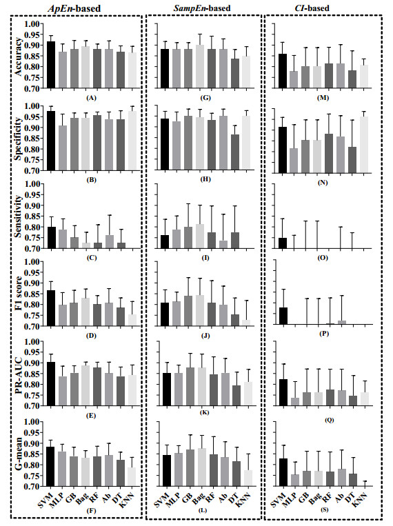
Vectorcardiography (VCG) was calculated from each 10-second ECG of CMD patients and healthy controls. Sample entropy (SampEn), approximate entropy (ApEn), and complexity index (CI) derived from multiscale entropy were extracted from ST-T segments of each lead in ECGs and VCGs. The most effective entropy subset was determined using the sequential backward selection algorithm under the intra-patient and inter-patient schemes, separately. Then, the corresponding optimal model was selected from eight machine learning models for each entropy feature based on five-fold cross-validations. Finally, the classification performance of SampEn-based, ApEn-based, and CI-based models was comprehensively evaluated and tested on a testing dataset to investigate the best one under each scheme.

Results
ApEn-based SVM model was validated as the optimal one under the intra-patient scheme, with all testing evaluation metrics over 0.8. Similarly, ApEn-based SVM model was selected as the best one under the intra-patient scheme, with major evaluation metrics over 0.8.

Conclusions
Entropies derived from ECGs and VCGs can effectively detect CMD under both intra-patient and inter-patient schemes. Our proposed models may provide the possibility of an ECG-based tool for non-invasive detection of CMD.
- coronary microvascular dysfunction (CMD),
- myocardial ischemia,
- entropy,
- machine learning,
- electrocardiogram (ECG),
- vectorcardiogram (VCG)
Citation: Xiaoye Zhao, Yinlan Gong, Lihua Xu, Ling Xia, Jucheng Zhang, Dingchang Zheng, Zongbi Yao, Xinjie Zhang, Haicheng Wei, Jun Jiang, Haipeng Liu, Jiandong Mao. Entropy-based reliable non-invasive detection of coronary microvascular dysfunction using machine learning algorithm[J]. Mathematical Biosciences and Engineering, 2023, 20(7): 13061-13085. doi: 10.3934/mbe.2023582

Related Papers:

Abstract

Purpose

Coronary microvascular dysfunction (CMD) is emerging as an important cause of myocardial ischemia, but there is a lack of a non-invasive method for reliable early detection of CMD.

Aim

To develop an electrocardiogram (ECG)-based machine learning algorithm for CMD detection that will lay the groundwork for patient-specific non-invasive early detection of CMD.

Methods

Vectorcardiography (VCG) was calculated from each 10-second ECG of CMD patients and healthy controls. Sample entropy (SampEn), approximate entropy (ApEn), and complexity index (CI) derived from multiscale entropy were extracted from ST-T segments of each lead in ECGs and VCGs. The most effective entropy subset was determined using the sequential backward selection algorithm under the intra-patient and inter-patient schemes, separately. Then, the corresponding optimal model was selected from eight machine learning models for each entropy feature based on five-fold cross-validations. Finally, the classification performance of SampEn-based, ApEn-based, and CI-based models was comprehensively evaluated and tested on a testing dataset to investigate the best one under each scheme.

Results

ApEn-based SVM model was validated as the optimal one under the intra-patient scheme, with all testing evaluation metrics over 0.8. Similarly, ApEn-based SVM model was selected as the best one under the intra-patient scheme, with major evaluation metrics over 0.8.

Conclusions

Entropies derived from ECGs and VCGs can effectively detect CMD under both intra-patient and inter-patient schemes. Our proposed models may provide the possibility of an ECG-based tool for non-invasive detection of CMD.

References

[1]	P. Severino, A. D'Amato, M. Pucci, F. Infusino, F. Adamo, L. I. Birtolo, et al., Ischemic heart disease pathophysiology paradigms overview: from paque activation to microvascular dysfunction, Int. J. Mol. Sci., 21 (2020), 8118. https://doi.org/10.3390/ijms21218118 doi: 10.3390/ijms21218118
[2]	A. E. Moran, M. H. Forouzanfar, G. A. Roth, G. A. Mensah, M. Ezzati, C. J. L. Murray, et al., Temporal trends in ischemic heart disease mortality in 21 world regions, 1980 to 2010, Circulation, 129 (2014), 1483-1492. https://doi.org/10.1161/CIRCULATIONAHA.113.004042 doi: 10.1161/CIRCULATIONAHA.113.004042
[3]	L. Dai, Y. Zang, G. Shou, L. Xia, Simulation of MCG signal in 2D cardiac tissue sheet with ischemic condition, in 2011 Computing in Cardiology, (2011), 21-24. Available from: http://cinc.mit.edu/archives/2011/pdf/0021.pdf.
[4]	J. Zhang, H. Li, Z. Pu, H. Liu, T. Huang, H. Cheng, et al., Early diagnosis of coronary microvascular dysfunction by myocardial contrast stress echocardiography, Math. Biosci. Eng., 20 (2023), 7845-7858. https://doi.org/10.3934/mbe.2023339 doi: 10.3934/mbe.2023339
[5]	F. Mangiacapra, M. M. Viscusi, G. Verolino, L. Paolucci, A. Nusca, R. Melfi, et al., Invasive assessment of coronary microvascular function, J. Clin. Med., 11 (2021), 228. https://doi.org/10.3390/jcm11010228 doi: 10.3390/jcm11010228
[6]	V. Kunadian, A. Chieffo, P. G. Camici, C. Berry, J. Escaned, A. H. E. M. Maas, et al., An EAPCI expert consensus document on Ischaemia with non-obstructive coronary arteries in collaboration with European society of cardiology working group on coronary pathophysiology & microcirculation endorsed by coronary vasomotor disorders international study group, Eur. Heart J., 41 (2020), 3504-3520. https://doi.org/10.1093/eurheartj/ehaa503 doi: 10.1093/eurheartj/ehaa503
[7]	S. H. Lee, D. Shin, J. M. Lee, T. P. van de Hoef, D. Hong, K. H. Choi, et al., Clinical relevance of Ischemia with nonobstructive coronary arteries according to coronary microvascular dysfunction, J. Am. Heart Assoc., 11 (2022), e025171. https://doi.org/doi:10.1161/JAHA.121.025171 doi: 10.1161/JAHA.121.025171
[8]	J. C. Kaski, F. Crea, B. J. Gersh, P. G. Camici, Reappraisal of ischemic heart disease, Circulation, 138 (2018), 1463-1480. https://doi.org/10.1161/CIRCULATIONAHA.118.031373 doi: 10.1161/CIRCULATIONAHA.118.031373
[9]	M. G. del Buono, R. A. Montone, M. Camilli, S. Carbone, J. Narula, C. J. Lavie, et al., Coronary microvascular dysfunction across the spectrum of cardiovascular diseases: JACC state-of-the-art review, J. Am. Coll. Cardiol., 78 (2021), 1352-1371. https://doi.org/10.1016/j.jacc.2021.07.042 doi: 10.1016/j.jacc.2021.07.042
[10]	J. Zhou, Y. Onuma, S. Garg, N. Kotoku, S. Kageyama, S. Masuda, et al., Angiography derived assessment of the coronary microcirculation: is it ready for prime time? Expert Rev. Cardiovasc. Ther., 20 (2022), 549-566. https://doi.org/10.1080/14779072.2022.2098117
[11]	C. N. B. Merz, C. J. Pepine, M. N. Walsh, J. L. F. P. G. Camici, W. M. Chilian, J. A. Clayton, et al., Ischemia and no obstructive coronary artery disease (INOCA), Circulation, 135 (2017), 1075-1092. https://doi.org/10.1161/CIRCULATIONAHA.116.024534 doi: 10.1161/CIRCULATIONAHA.116.024534
[12]	P. Ong, P. G. Camici, J. F. Beltrame, F. Crea, H. Shimokawa, U. Sechtem, et al., International standardization of diagnostic criteria for microvascular angina, Int. J. Cardiol., 250 (2018), 16-20. https://doi.org/10.1016/j.ijcard.2017.08.068 doi: 10.1016/j.ijcard.2017.08.068
[13]	B. Tjoe, L. Barsky, J. Wei, B. Samuels, B. Azarbal, C. N. B. Merz, et al., Coronary microvascular dysfunction: considerations for diagnosis and treatment, Cleve. Clin. J. Med., 88 (2021), 561-571. https://doi.org/doi:10.3949/ccjm.88a.20140 doi: 10.3949/ccjm.88a.20140
[14]	M. A. Marinescu, A. I. Löffler, M. Ouellette, L. Smith, C. M. Kramer, J. M. Bourque, Coronary microvascular dysfunction, microvascular angina, and treatment strategies, JACC Cardiovasc. Imaging, 8 (2015), 210-220. https://doi.org/10.1016/j.jcmg.2014.12.008 doi: 10.1016/j.jcmg.2014.12.008
[15]	V. M. Pereyra, A. Seitz, H. Mahrholdt, R. Bekeredjian, U. Sechtem, P. Ong, Coronary microvascular dysfunction in patients with mild-to-moderate aortic stenosis - insights from intracoronary acetylcholine testing, Int. J. Cardiol. Heart Vasc., 31 (2020), 100658. https://doi.org/10.1016/j.ijcha.2020.100658 doi: 10.1016/j.ijcha.2020.100658
[16]	E. Aribas, J. E. Roeters van Lennep, S. E. Elias-Smale, J. J. Piek, M. Roos, F. Ahmadizar, et al., Prevalence of microvascular angina among patients with stable symptoms in the absence of obstructive coronary artery disease: a systematic review, Cardiovasc. Res., 118 (2022), 763-771. https://doi.org/10.1093/cvr/cvab061 doi: 10.1093/cvr/cvab061
[17]	Branch of Cardiovascular Physicians, Chinese Medical Doctor Association, 2020 expert consensus on the prevention and treatment of heart failure after myocardial infarction, Chin. Circ. J., 35 (2020), 1166-1180. Available from: https://corestarbio.com/uploadfile/1669779085_2.pdf.
[18]	H. Liu, S. Ou, P. Liu, Y. Xu, Y. Gong, L. Xia, et al., Effect of microcirculatory resistance on coronary blood flow and instantaneous wave-free ratio: a computational study, Comput. Methods Programs Biomed., 196 (2020), 105632. https://doi.org/10.1016/j.cmpb.2020.105632 doi: 10.1016/j.cmpb.2020.105632
[19]	J. Knuuti, W. Wijns, A. Saraste, D. Capodanno, E. Barbato, C. Funck-Brentano, et al., 2019 ESC Guidelines for the diagnosis and management of chronic coronary syndromes, Eur. Heart J., 41 (2019), 407-477. https://doi.org/10.1093/eurheartj/ehz425 doi: 10.1093/eurheartj/ehz425
[20]	Y. Geng, X. Wu, H. Liu, D. Zheng, L. Xia, Index of microcirculatory resistance: state-of-the-art and potential applications in computational simulation of coronary artery disease, J. Zhejiang Univ. Sci. B, 23 (2022), 123-140. https://doi.org/10.1631/jzus.B2100425 doi: 10.1631/jzus.B2100425
[21]	P. G. Camici, G. d'Amati, O. Rimoldi, Coronary microvascular dysfunction: mechanisms and functional assessment, Nat. Rev. Cardiol., 12 (2015), 48-62. https://doi.org/10.1038/nrcardio.2014.160 doi: 10.1038/nrcardio.2014.160
[22]	J. D. Sara, A. Sugrue, V. Kremen, B. Qiang, Y. Sapir, Z. I. Attia, et al., Electrocardiographic predictors of coronary microvascular dysfunction in patients with non-obstructive coronary artery disease: utility of a novel T wave analysis program, Int. J. Cardiol., 203 (2016), 601-606. https://doi.org/10.1016/j.ijcard.2015.10.228 doi: 10.1016/j.ijcard.2015.10.228
[23]	J. Herrmann, J. C. Kaski, A. Lerman, Coronary microvascular dysfunction in the clinical setting: from mystery to reality, Eur. Heart J., 33 (2012), 2771-2783. https://doi.org/10.1093/eurheartj/ehs246 doi: 10.1093/eurheartj/ehs246
[24]	Z. Zhou, Y. Liu, Z. Wang, Y. Wang, J. Zhang, C. Yang, The value of standard deviation of normal RR Interval in predicting coronary microvascular dysfunction in patients with ischemia with non obstructive coronary arteries (in Chinese), Chin. Circ. J., 37 (2022), 804-809. https://doi.org/10.3969/j.issn.1000-3614.2022.08.008 doi: 10.3969/j.issn.1000-3614.2022.08.008
[25]	E. Fabris, A. W. J. van't Hof, 7- Angiography and electrocardiography (ECG) for the assessment of coronary microvascular obstruction, in Coronary Microvascular Obstruction in Acute Myocardial Infarction (eds. G. Niccoli and I. Eitel), New York: Academic Press, (2018), 109-126.
[26]	P. Ong, A. Athanasiadis, S. Hill, T. Schäufele, H. Mahrholdt, U. Sechtem, Coronary microvascular dysfunction assessed by intracoronary acetylcholine provocation testing is a frequent cause of ischemia and angina in patients with exercise-induced electrocardiographic changes and unobstructed coronary arteries, Clin. Cardiol., 37 (2014), 462-467. https://doi.org/10.1002/clc.22282 doi: 10.1002/clc.22282
[27]	N. Dose, M. M. Michelsen, N. D. Mygind, A. Pena, C. Ellervik, P. R. Hansen, et al., Ventricular repolarization alterations in women with angina pectoris and suspected coronary microvascular dysfunction, J. Electrocardiol., 51 (2018), 15-20. https://doi.org/10.1016/j.jelectrocard.2017.08.017 doi: 10.1016/j.jelectrocard.2017.08.017
[28]	J. D. Sara, R. J. Lennon, M. J. Ackerman, P. A. Friedman, P. A. Noseworthy, A. Lerman, Coronary microvascular dysfunction is associated with baseline QTc prolongation amongst patients with chest pain and non-obstructive coronary artery disease, J. Electrocardiol., 49 (2016), 87-93. https://doi.org/10.1016/j.jelectrocard.2015.10.006 doi: 10.1016/j.jelectrocard.2015.10.006
[29]	R. Alizadehsani, M. Abdar, M. Roshanzamir, A. Khosravi, P. M. Kebria, F. Khozeimeh, et al., Machine learning-based coronary artery disease diagnosis: a comprehensive review, Comput. Biol. Med., 111 (2019), 103346. https://doi.org/10.1016/j.compbiomed.2019.103346 doi: 10.1016/j.compbiomed.2019.103346
[30]	J. S. Richman, J. R. Moorman, Physiological time-series analysis using approximate entropy and sample entropy, Am. J. Physiol. Heart Circ. Physiol., 278 (2000), H2039-H2049. https://doi.org/10.1152/ajpheart.2000.278.6.H2039 doi: 10.1152/ajpheart.2000.278.6.H2039
[31]	R. K. Udhayakumar, C. Karmakar, M. Palaniswami, Entropy profiling to detect ST change in heart rate variability signals, in 2019 41st Annual International Conference of the IEEE Engineering in Medicine and Biology Society (EMBC), (2019), 4588-4591. https://doi.org/10.1109/EMBC.2019.8857297
[32]	H. Rabbani, M. P. Mahjoob, E. Farahabadi, A. Farahabadi, A. M. Dehnavi, Ischemia detection by electrocardiogram in wavelet domain using entropy measure, J. Res. Med. Sci., 16 (2011), 1473-1482. Available from: https://www.researchgate.net/publication/230843943.
[33]	J. Liu, C. Zhang, T. Ristaniemi, F. Cong, Detection of myocardial infarction from multi-lead ECG using dual-Q tunable Q-factor wavelet transform, in 2019 41st Annual International Conference of the IEEE Engineering in Medicine and Biology Society (EMBC), 2019 (2019), 1496-1499. https://doi.org/10.1109/EMBC.2019.8857775
[34]	C. Chen, Y. Jin, I. L. Lo, H. Zhao, B. Sun, Q. Zhao, et al., Complexity change in cardiovascular disease, Int. J. Biol. Sci., 13 (2017), 1320-1328. https://doi.org/10.7150/ijbs.19462 doi: 10.7150/ijbs.19462
[35]	J. M. Ahn, S. Arora, O. G. Solberg, O. Angerås, K. Rolid, M. Rafique, et al., Prognostic value of comprehensive intracoronary physiology assessment early after heart transplantation, Eur. Heart J., 42 (2021), 4918-4929. https://doi.org/10.1093/eurheartj/ehab568 doi: 10.1093/eurheartj/ehab568
[36]	E. A. P. Alday, A. Gu, A. J. Shah, C. Robichaux, A. K. I. Wong, C. Liu, et al., Classification of 12-lead ECGs: the physioNet/computing in cardiology challenge 2020, Physiol. Meas., 41 (2021), 124003-124003. https://doi.org/10.1088/1361-6579/abc960 doi: 10.1088/1361-6579/abc960
[37]	X. Zhao, J. Zhang, Y. Gong, L. Xu, H. Liu, S. Wei, et al., Reliable detection of myocardial ischemia using machine learning based on temporal-spatial characteristics of electrocardiogram and vectorcardiogram, Front. Physiol., 13 (2022). https://doi.org/10.3389/fphys.2022.854191
[38]	C. E. Kossmann, D. Brody, G. Burch, H. Hecht, F. Johnston, C. Kay, et al., Report of committee on electrocardiography, American Heart Association, Recommendations for standardization of leads and of specifications for instruments in electrocardiography and vectorcardiography, Circulation, 35 (1967), 583-602. https://doi.org/10.1161/01.cir.35.3.583 doi: 10.1161/01.cir.35.3.583
[39]	J. A. Kors, G. van Herpen, A. C. Sittig, J. H. van Bemmel, Reconstruction of the Frank vectorcardiogram from standard electrocardiographic leads: diagnostic comparison of different methods, Eur. Heart J., 11 (1990), 1083-1092. https://doi.org/10.1093/oxfordjournals.eurheartj.a059647 doi: 10.1093/oxfordjournals.eurheartj.a059647
[40]	J. Song, H. Yan, Z. Xiao, X. Yang, X. Zhang, A robust and efficientalgorithm for ST–T complex detection in electrocardiograms, J. Mech. Med. Biol., 11 (2012), 1103-1111. https://doi.org/10.1142/s0219519411004198 doi: 10.1142/s0219519411004198
[41]	A. Molina-Picó, D. Cuesta-Frau, M. Aboy, C. Crespo, P. Miró-Martínez, S. Oltra-Crespo, Comparative study of approximate entropy and sample entropy robustness to spikes, Artif. Intell. Med., 53 (2011), 97-106. https://doi.org/10.1016/j.artmed.2011.06.007 doi: 10.1016/j.artmed.2011.06.007
[42]	M. A. Busa, R. E. A. van Emmerik, Multiscale entropy: a tool for understanding the complexity of postural control, J. Sport Health Sci., 5 (2016), 44-51. https://doi.org/10.1016/j.jshs.2016.01.018 doi: 10.1016/j.jshs.2016.01.018
[43]	J. M. Yentes, N. Hunt, K. K. Schmid, J. P. Kaipust, D. McGrath, N. Stergiou, The appropriate use of approximate entropy and sample entropy with short data sets, Ann. Biomed. Eng., 41 (2013), 349-365. https://doi.org/10.1007/s10439-012-0668-3 doi: 10.1007/s10439-012-0668-3
[44]	D. U. Uguz, F. Berief, S. Leonhardt, C. H. Antink, Classification of 12-lead ECGs using gradient boosting on features acquired with domain-specific and domain-agnostic methods, in 2020 Computing in Cardiology, (2020), 1-4. https://doi.org/10.22489/CinC.2020.363
[45]	A. U. Haq, J. Li, M. H. Memon, M. H. Memon, J. Khan, S. M. Marium, Heart disease prediction system using model of machine learning and sequential backward selection algorithm for features selection, in 2019 IEEE 5th International Conference for Convergence in Technology (I2CT), 2019. https://doi.org/10.1109/I2CT45611.2019.9033683
[46]	M. Alnowami, F. Abolaban, E. Taha, A wrapper-based feature selection approach to investigate potential biomarkers for early detection of breast cancer, J. Radiat. Res. Appl. Sci., 15 (2022), 104-110. https://doi.org/10.1016/j.jrras.2022.01.003 doi: 10.1016/j.jrras.2022.01.003
[47]	L. Li, X. Sui, J. Lian, F. Yu, Y. Zhou, Vehicle interaction behavior prediction with self-attention, Sensors, 22 (2022), 429. https://doi.org/10.3390/s22020429 doi: 10.3390/s22020429
[48]	C. Xie, R. Du, J. W. K. Ho, H. H. Pang, K. W. H. Chiu, E. Y. P. Lee, et al., Effect of machine learning re-sampling techniques for imbalanced datasets in 18F-FDG PET-based radiomics model on prognostication performance in cohorts of head and neck cancer patients, Eur. J. Nucl. Med. Mol. Imaging, 47 (2020), 2826-2835. https://doi.org/10.1007/s00259-020-04756-4 doi: 10.1007/s00259-020-04756-4
[49]	T. Saito, M. Rehmsmeier, The precision-recall plot is more informative than the ROC plot when evaluating binary classifiers on imbalanced datasets, PLoS One, 10 (2015), e0118432. https://doi.org/10.1371/journal.pone.0118432 doi: 10.1371/journal.pone.0118432
[50]	S. Ansari, N. Farzaneh, M. Duda, K. Horan, H. B. Andersson, Z. D. Goldberger, et al., A review of automated methods for detection of myocardial ischemia and infarction using electrocardiogram and electronic health records, IEEE Rev. Biomed. Eng., 10 (2017), 264-298. https://doi.org/10.1109/RBME.2017.2757953 doi: 10.1109/RBME.2017.2757953
[51]	R. Correa, P. D. Arini, L. S. Correa, M. Valentinuzzi, E. Laciar, Novel technique for ST-T interval characterization in patients with acute myocardial ischemia, Comput. Biol. Med., 50 (2014), 49-55. https://doi.org/10.1016/j.compbiomed.2014.04.009 doi: 10.1016/j.compbiomed.2014.04.009
[52]	Y. L. Zang, L. Xia, Cellular mechanism of cardiac alternans: an unresolved chicken or egg problem, J. Zhejiang Univ. Sci. B, 15 (2014), 201-211. https://doi.org/10.1631/jzus.B1300177 doi: 10.1631/jzus.B1300177
[53]	M. J. Janse, A. L. Wit, Electrophysiological mechanisms of ventricular arrhythmias resulting from myocardial ischemia and infarction, Physiol. Rev., 69 (1989), 1049-1169. https://doi.org/10.1152/physrev.1989.69.4.1049 doi: 10.1152/physrev.1989.69.4.1049
[54]	C. C. ter Haar, A. C. Maan, S. G Warren, M. Ringborn, B. M. Horáček, M. J. Schalij, et al., Difference vectors to describe dynamics of the ST segment and the ventricular gradient in acute ischemia, J. Electrocardiol., 46 (2013), 302-311. https://doi.org/10.1016/j.jelectrocard.2013.04.004 doi: 10.1016/j.jelectrocard.2013.04.004
[55]	A. Feeny, L. G. Tereshchenko, Beat-to-beat determinants of the beat-to-beat temporal and spatial variability of repolarization, J. Electrocardiol., 49 (2016), 417-422. https://doi.org/10.1016/j.jelectrocard.2016.01.007 doi: 10.1016/j.jelectrocard.2016.01.007
[56]	M. Wei, J. Z. Song, H. Yan, Electrocardiogram ST-segment morphology variability analysis base on correlation coefficient entropy and inverse correlation coefficient entropy, Appl. Mech. Mater., 195-196 (2012), 550-554. https://doi.org/10.4028/www.scientific.net/AMM.195-196.550
[57]	M. Ferrario, M. G. Signorini, G. Magenes, S. Cerutti, Comparison of entropy-based regularity estimators: application to the fetal heart rate signal for the identification of fetal distress, IEEE Trans. Biomed. Eng., 53 (2006), 119-125. https://doi.org/10.1109/TBME.2005.859809 doi: 10.1109/TBME.2005.859809
[58]	S. D. Fihn, J. C. Blankenship, K. P. Alexander, J. A. Bittl, J. G. Byrne, B. J. Fletcher, et al., 2014 ACC/AHA/AATS/PCNA/SCAI/STS Focused Update of the Guideline for the Diagnosis and Management of Patients With Stable Ischemic Heart Disease: A Report of the American College of Cardiology/American Heart Association Task Force on Practice Guidelines, and the American Association for Thoracic Surgery, Preventive Cardiovascular Nurses Association, Society for Cardiovascular Angiography and Interventions, and Society of Thoracic Surgeons, J. Am. Coll. Cardiol., 64 (2014), 1929-1949. https://doi.org/10.1016/j.jacc.2014.07.017 doi: 10.1016/j.jacc.2014.07.017
[59]	H. A. Mayala, W. Yan, H. Jing, S. Liu, G. Yi, C. Qin, et al., Clinical characteristics and biomarkers of coronary microvascular dysfunction and obstructive coronary artery disease, J. Int. Med. Res., 47 (2019), 6149-6159. https://doi.org/10.1177/0300060519859134 doi: 10.1177/0300060519859134

Reader Comments

Your name:*

Email:*
© 2023 the Author(s), licensee AIMS Press. This is an open access article distributed under the terms of the Creative Commons Attribution License (http://creativecommons.org/licenses/by/4.0)