Research on user recruitment algorithms based on user trajectory prediction with sparse mobile crowd sensing

Jing Zhang; Qianqian Wang; Ding Lang; Yuguang Xu; Hong-an Li; Xuewen Li; Jing Zhang; Qianqian Wang; Ding Lang; Yuguang Xu; Hong-an Li; Xuewen Li

doi:10.3934/mbe.2023533

Mathematical Biosciences and Engineering

2023, Volume 20, Issue 7: 11998-12023. doi: 10.3934/mbe.2023533

Previous Article Next Article

Research article Special Issues

Research on user recruitment algorithms based on user trajectory prediction with sparse mobile crowd sensing

1.
School of Computer Science and Technology, Xi'an University of Science and Technology, Xian 710600, China
2.
School of Energy Enginnering, Xi'an University of Science and Technology, Xian 710600, China
3.
School of Safety Science and Engineering, Xi'an University of Science and Technology, Xian 710600, China

Academic Editor: Yiu-ming Cheung

Received: 10 February 2023 Revised: 13 April 2023 Accepted: 24 April 2023 Published: 12 May 2023

Sparse mobile crowd sensing saves perception cost by recruiting a small number of users to perceive data from a small number of sub-regions, and then inferring data from the remaining sub-regions. The data collected by different people on their respective trajectories have different values, and we can select participants who can collect high-value data based on their trajectory predictions. In this paper, we study two aspects of user trajectory prediction and user recruitment. First, we propose an STGCN-GRU user trajectory prediction algorithm, which uses the STGCN algorithm to extract features related to temporal and spatial information from the trajectory map, and then inputs the feature sequences into GRU for trajectory prediction, and this algorithm improves the accuracy of user trajectory prediction. Second, an ADQN (action DQN) user recruitment algorithm is proposed.The ADQN algorithm improves the objective function in DQN on the idea of reinforcement learning. The action with the maximum input value is found from the Q network, and then the output value of the objective function of the corresponding action Q network is found. This reduces the overestimation problem that occurs in Q networks and improves the accuracy of user recruitment. The experimental results show that the evaluation metrics FDE and ADE of the STGCN-GRU algorithm proposed in this paper are better than other representative algorithms. And the experiments on two real datasets verify the effectiveness of the ADQN user selection algorithm, which can effectively improve the accuracy of data inference under budget constraints.
- sparse mobile crowd sensing,
- STGCN-GRU,
- user selection,
- reinforcement learning
Citation: Jing Zhang, Qianqian Wang, Ding Lang, Yuguang Xu, Hong-an Li, Xuewen Li. Research on user recruitment algorithms based on user trajectory prediction with sparse mobile crowd sensing[J]. Mathematical Biosciences and Engineering, 2023, 20(7): 11998-12023. doi: 10.3934/mbe.2023533

Related Papers:

Abstract

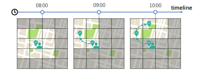
Sparse mobile crowd sensing saves perception cost by recruiting a small number of users to perceive data from a small number of sub-regions, and then inferring data from the remaining sub-regions. The data collected by different people on their respective trajectories have different values, and we can select participants who can collect high-value data based on their trajectory predictions. In this paper, we study two aspects of user trajectory prediction and user recruitment. First, we propose an STGCN-GRU user trajectory prediction algorithm, which uses the STGCN algorithm to extract features related to temporal and spatial information from the trajectory map, and then inputs the feature sequences into GRU for trajectory prediction, and this algorithm improves the accuracy of user trajectory prediction. Second, an ADQN (action DQN) user recruitment algorithm is proposed.The ADQN algorithm improves the objective function in DQN on the idea of reinforcement learning. The action with the maximum input value is found from the Q network, and then the output value of the objective function of the corresponding action Q network is found. This reduces the overestimation problem that occurs in Q networks and improves the accuracy of user recruitment. The experimental results show that the evaluation metrics FDE and ADE of the STGCN-GRU algorithm proposed in this paper are better than other representative algorithms. And the experiments on two real datasets verify the effectiveness of the ADQN user selection algorithm, which can effectively improve the accuracy of data inference under budget constraints.

References

[1]	F. Abbondati, S. A. Biancardo, R. Veropalumbo, G. Dell'Acqua, Surface monitoring of road pavements using mobile crowdsensing technology, Measurement, 171 (2021), 108763. https://doi.org/10.1016/j.measurement.2020.108763 doi: 10.1016/j.measurement.2020.108763
[2]	Y. Huang, H. Chen, G. Ma, K. Lin, Z. Ni, N. Yan, et al., OPAT: Optimized allocation of time-dependent tasks for mobile crowdsensing, IEEE Trans. Ind. Inf., 18 (2021), 2476–2485. https://doi.org/10.1109/TII.2021.3094527 doi: 10.1109/TII.2021.3094527
[3]	T. Tang, L. Cui, Z. Yin, S. Hu, L. Fu, Spatiotemporal characteristic aware task allocation strategy using sparse user data in mobile crowdsensing, Wireless Networks, 29 (2023), 459–474. https://doi.org/10.1007/s11276-022-03138-y doi: 10.1007/s11276-022-03138-y
[4]	S. He, K. G. Shin, Steering crowdsourced signal map construction via Bayesian compressive sensing, in IEEE INFOCOM 2018-IEEE Conference on Computer Communications, (2018), 1016–1024. https://doi.org/10.1109/INFOCOM.2018.8485972
[5]	L. Wang, D. Zhang, Y. Wang, C. Chen, X. Han, A. M'hamed, Sparse mobile crowdsensing: challenges and opportunities, IEEE Commun. Mag., 54 (2016), 161–167. https://doi.org/10.1109/MCOM.2016.7509395 doi: 10.1109/MCOM.2016.7509395
[6]	W. Liu, Y. Yang, E. Wang, J. Wu, User recruitment for enhancing data inference accuracy in sparse mobile crowdsensing, IEEE Internet Things J., 7 (2019), 1802–1814. https://doi.org/10.1109/JIOT.2019.2957399 doi: 10.1109/JIOT.2019.2957399
[7]	C. Tu, Z. Yu, L. Han, W. Zhu, F. Huang, L. Wang, Direct participant recruitment strategy in sparse mobile crowd sensing, Chin. J. Comput., 45 (2022), 1539–1556. https://doi.org/10.11897/SP.J.1016.2022.01539 doi: 10.11897/SP.J.1016.2022.01539
[8]	L. Han, Z. Yu, L. Wang, Z. Yu, B. Guo, Keeping cell selection model up-to-date to adapt to time-dependent environment in sparse mobile crowdsensing, IEEE Internet Things J., 8 (2021), 13914–13925. https://doi.org/10.1109/JIOT.2021.3068415 doi: 10.1109/JIOT.2021.3068415
[9]	T. Liu, Y. Zhu, Y. Yang, F. Ye, $ALC^{2}$: When active learning meets compressive crowdsensing for urban air pollution monitoring, IEEE Internet Things J., 6 (2019), 9427–9438. https://doi.org/10.1109/JIOT.2019.2939552 doi: 10.1109/JIOT.2019.2939552
[10]	Y. Zhu, Z. Li, H. Zhu, M. Li, Q. Zhang, A compressive sensing approach to urban traffic estimation with probe vehicles, IEEE Trans. Mobile Comput., 12 (2012), 2289–2302. https://doi.org/10.1109/TMC.2012.205 doi: 10.1109/TMC.2012.205
[11]	J. Wang, F. Wang, Y. Wang, D. Zhang, L. Wang, Z. Qiu, et al., Social-network-assisted worker recruitment in mobile crowd sensing, IEEE Trans. Mobile Comput., 18 (2018), 1661–1673. https://doi.org/10.1109/TMC.2018.2865355 doi: 10.1109/TMC.2018.2865355
[12]	H. Li, T. Li, W. Wang, Y. Wang, Dynamic participant selection for large-scale mobile crowd sensing, IEEE Trans. Mobile Comput., 18 (2018), 2842–2855. https://doi.org/10.1109/TMC.2018.2884945 doi: 10.1109/TMC.2018.2884945
[13]	H. Gao, C. Liu, J. Tang, D. Yang, P. Hui, W. Wang, Online quality-aware incentive mechanism for mobile crowd sensing with extra bonus, IEEE Trans. Mobile Comput., 18 (2018), 2589–2603. https://doi.org/10.1109/TMC.2018.2877459 doi: 10.1109/TMC.2018.2877459
[14]	L. Pu, X. Chen, J. Xu, X. Fu, Crowd foraging: A QoS-oriented self-organized mobile crowdsourcing framework over opportunistic networks, IEEE J. Sel. Areas Commun., 35 (2017), 848–862. https://doi.org/10.1109/JSAC.2017.2679598 doi: 10.1109/JSAC.2017.2679598
[15]	J. Li, J. Wu, Y. Zhu, Selecting optimal mobile users for long-term environmental monitoring by crowdsourcing, in Proceedings of the International Symposium on Quality of Service, (2019), 1–10. https://doi.org/10.1145/3326285.3329043
[16]	Q. Yang, Y. Chen, M. Guizani, G. M. Lee, Spatiotemporal location differential privacy for sparse mobile crowdsensing, in 2021 International Wireless Communications and Mobile Computing (IWCMC), (2021), 1734–1741. https://doi.org/10.1109/IWCMC51323.2021.9498951
[17]	J. Shen, J. Peng, L. Shao, Submodular trajectories for better motion segmentation in videos, IEEE Trans. Image Process., 27 (2018), 2688–2700. https://doi.org/10.1109/TIP.2018.2795740 doi: 10.1109/TIP.2018.2795740
[18]	D. Yao, C. Zhang, Z. Zhu, J. Huang, J. Bi, Trajectory clustering via deep representation learning, in 2017 international joint conference on neural networks (IJCNN), (2017), 3880–3887. https://doi.org/10.1109/IJCNN.2017.7966345
[19]	J. Quehl, H. Hu, S. Wirges, M. Lauer, An approach to vehicle trajectory prediction using automatically generated traffic maps, in 2018 IEEE Intelligent Vehicles Symposium (IV), (2018), 544–549. https://doi.org/10.1109/IVS.2018.8500535
[20]	H. Xue, D. Q. Huynh, M. Reynolds, SS-LSTM: A hierarchical LSTM model for pedestrian trajectory prediction, in 2018 IEEE Winter Conference on Applications of Computer Vision (WACV), (2018), 1186–1194. https://doi.org/10.1109/WACV.2018.00135
[21]	G. Xie, H. Gao, L. Qian, B. Huang, K. Li, J. Wang, Vehicle trajectory prediction by integrating physics-and maneuver-based approaches using interactive multiple models, IEEE Trans. Ind. Electron., 65 (2017), 5999–6008. https://doi.org/10.1109/TIE.2017.2782236 doi: 10.1109/TIE.2017.2782236
[22]	T. Fernando, S. Denman, S. Sridharan, C. Fookes, Tracking by prediction: A deep generative model for mutli-person localisation and tracking, in 2018 IEEE Winter conference on applications of computer vision (WACV), (2018), 1122–1132. https://doi.org/10.1109/WACV.2018.00128
[23]	H. Woo, Y. Ji, H. Kono, Y. Tamura, Y. Kuroda, T. Sugano, et al., Lane-change detection based on vehicle-trajectory prediction, IEEE Rob. Autom. Lett., 2 (2017), 1109–1116. https://doi.org/10.1109/LRA.2017.2660543 doi: 10.1109/LRA.2017.2660543
[24]	N. Deo, A. Rangesh, M. M. Trivedi, How would surround vehicles move? A unified framework for maneuver classification and motion prediction, IEEE Trans. Intell. Veh., 3 (2018), 129–140. https://doi.org/10.1109/TIV.2018.2804159 doi: 10.1109/TIV.2018.2804159
[25]	B. Yu, H. Yin, Z. Zhu, Spatio-temporal graph convolutional networks: A deep learning framework for traffic forecasting, preprint, arXiv: 1709.04875. https://doi.org/10.48550/arXiv.1709.04875
[26]	S. Guo, Y. Lin, N. Feng, C. Song, H. Wan, Attention based spatial-temporal graph convolutional networks for traffic flow forecasting, in Proceedings of the AAAI Conference on Artificial Intelligence, 33 (2019), 922–929. https://doi.org/10.1609/aaai.v33i01.3301922
[27]	C. Song, Y. Lin, S. Guo, H. Wan, Spatial-temporal synchronous graph convolutional networks: A new framework for spatial-temporal network data forecasting, in Proceedings of the AAAI Conference on Artificial Intelligence, 34 (2020), 914–921. https://doi.org/10.1609/aaai.v34i01.5438
[28]	X. Luo, X. Chen, L. Shou, K. Chen, Y. Wu, Semantic trajectory extraction framework for indoor space, Tsinghua Sci. Technol., 59 (2019), 186–193. https://doi.org/10.16511/j.cnki.qhdxxb.2018.26.047 doi: 10.16511/j.cnki.qhdxxb.2018.26.047
[29]	L. Kaiser, M. Babaeizadeh, P. Milos, B. Osinski, R. H. Campbell, K. Czechowski, et al., Model-based reinforcement learning for atari, preprint, arXiv: 1903.00374. https://doi.org/10.48550/arXiv.1903.00374
[30]	V. Mnih, K. Kavukcuoglu, D. Silver, A. Graves, I. Antonoglou, D. Wierstra, et al., Playing atari with deep reinforcement learning, preprint, arXiv: 1312.5602. https://doi.org/10.48550/arXiv.1312.5602
[31]	D. Silver, A. Huang, C. J. Maddison, A. Guez, L. Sifre, G. Van Den Driessche, et al., Mastering the game of go with deep neural networks and tree search, Nature, 529 (2016), 484–489. https://doi.org/10.1038/nature16961 doi: 10.1038/nature16961
[32]	M. Hausknecht, P. Stone, Deep recurrent q-learning for partially observable mdps, in 2015 AAAI Fall Symposium Series, 2015 (2015). https://doi.org/10.48550/arXiv.1507.06527
[33]	G. Lample, D. S. Chaplot, Playing fps games with deep reinforcement learning, in Proceedings of the AAAI Conference on Artificial Intelligence, 31 (2017). https://doi.org/10.1609/aaai.v31i1.10827
[34]	H. Li, T. Li, F. Li, S. Yang, Y. Wang, Multi-expertise aware participant selection in mobile crowd sensing via online learning, in 2018 IEEE 15th International Conference on Mobile Ad Hoc and Sensor Systems (MASS), (2018), 433–441. https://doi.org/10.1109/MASS.2018.00067
[35]	X. Zhang, X. Gong, Online data quality learning for quality-aware crowdsensing, in 2019 16th Annual IEEE International Conference on Sensing, Communication, and Networking (SECON), (2019), 1–9. https://doi.org/10.1109/SAHCN.2019.8824861
[36]	H. Zhao, M. Xiao, J. Wu, Y. Xu, H. Huang, S. Zhang, Differentially private unknown worker recruitment for mobile crowdsensing using multi-armed bandits, IEEE Trans. Mobile Comput., 20 (2021), 2779–2794. https://doi.org/10.1109/TMC.2020.2990221 doi: 10.1109/TMC.2020.2990221
[37]	G. Gao, J. Wu, M. Xiao G. Chen, Combinatorial multi-armed bandit based unknown worker recruitment in heterogeneous crowdsensing, in IEEE INFOCOM 2020 - IEEE Conference on Computer Communications, (2020), 179–188. https://doi.org/10.1109/INFOCOM41043.2020.9155518
[38]	L. Xiao, T. Chen, C. Xie, H. Dai H. V. Poor, Mobile crowdsensing games in vehicular networks, IEEE Trans. Veh. Technol., 67 (2018), 1535–1545. https://doi.org/10.1109/TVT.2016.2647624 doi: 10.1109/TVT.2016.2647624
[39]	A. Alahi, K. Goel, V. Ramanathan, A. Robicquet, F. F. Li, S. Savarese, Social lstm: Human trajectory prediction in crowded spaces, in Proceedings of the IEEE Conference on Computer Vision and Pattern Recognition (CVPR), (2016), 961–971. https://doi.org/10.1109/CVPR.2016.110

Reader Comments

Your name:*

Email:*
© 2023 the Author(s), licensee AIMS Press. This is an open access article distributed under the terms of the Creative Commons Attribution License (http://creativecommons.org/licenses/by/4.0)