Bayesian estimation of parameters in viral dynamics models with antiviral effect of interferons in a cell culture

Miguel Ángel Rodríguez-Parra; Cruz Vargas-De-León; Flaviano Godinez-Jaimes; Celia Martinez-Lázaro; Miguel Ángel Rodríguez-Parra; Cruz Vargas-De-León; Flaviano Godinez-Jaimes; Celia Martinez-Lázaro

doi:10.3934/mbe.2023488

Mathematical Biosciences and Engineering

2023, Volume 20, Issue 6: 11033-11062. doi: 10.3934/mbe.2023488

Previous Article Next Article

Research article

Bayesian estimation of parameters in viral dynamics models with antiviral effect of interferons in a cell culture

1.
Facultad de Matemáticas, Universidad Autónoma de Guerrero, Ciudad Universitaria s/n Chilpancingo, Guerrero, México
2.
División de Investigación, Hospital Juárez de México, Ciudad de México 07760, México
3.
Sección de Estudios de Posgrado, Escuela Superior de Medicina, Instituto Politécnico Nacional, Ciudad de México 11340, México

Academic Editor: Hao Wang

Received: 06 March 2023 Revised: 17 April 2023 Accepted: 18 April 2023 Published: 23 April 2023

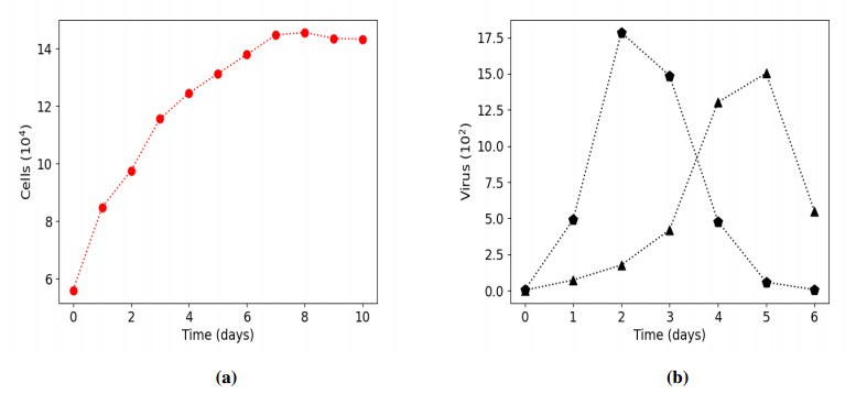
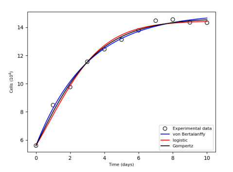
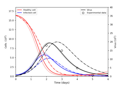
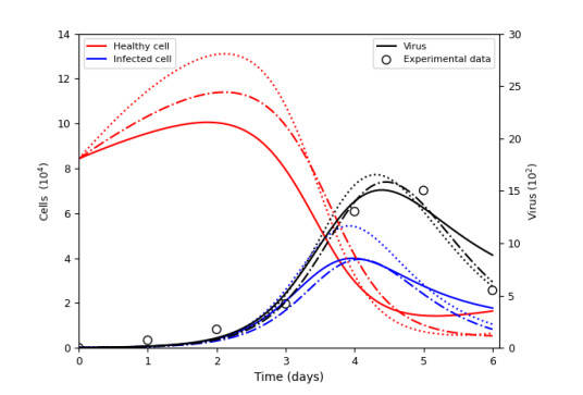
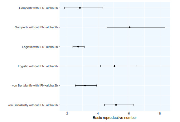
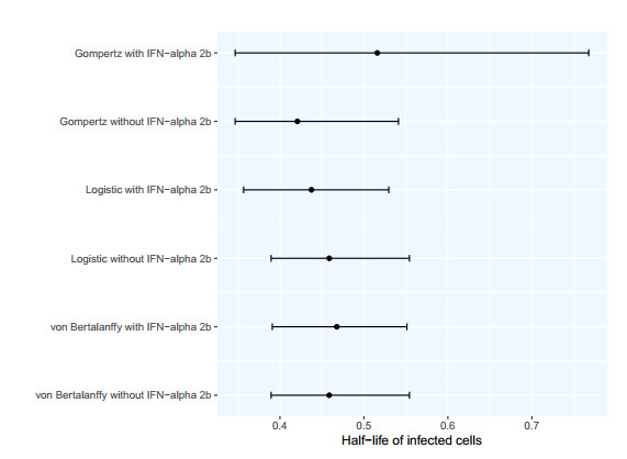
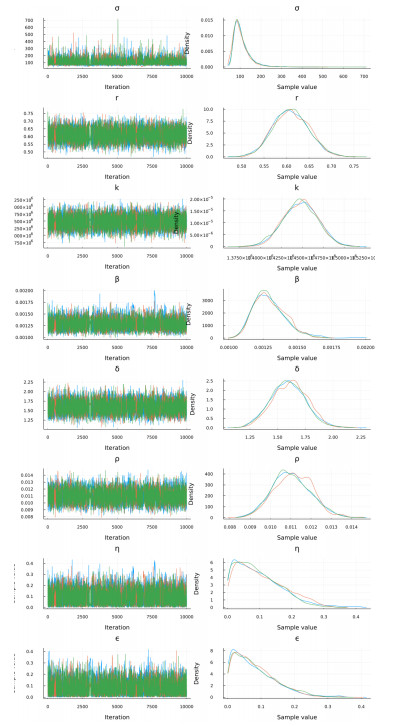
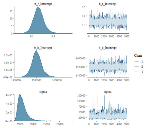
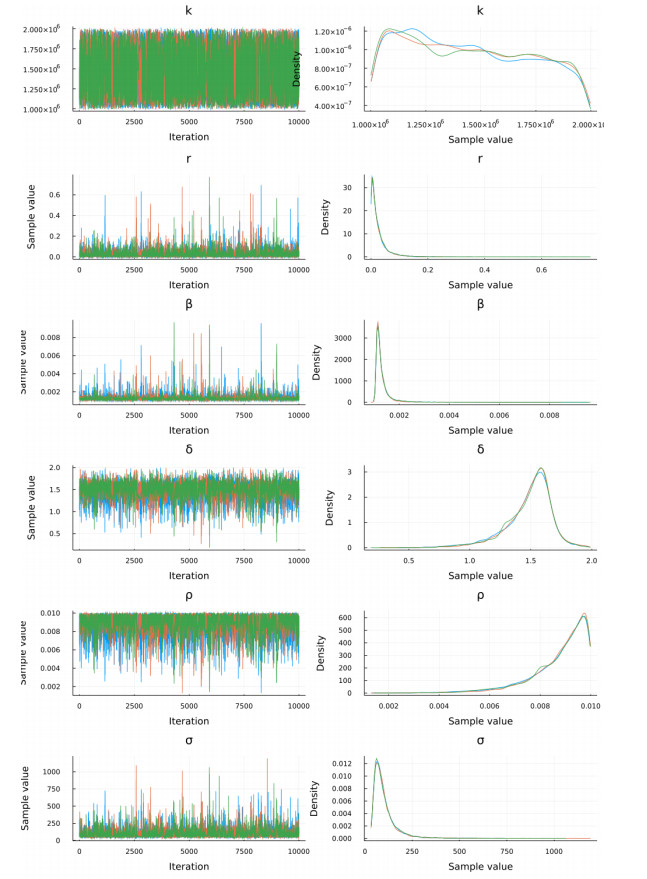
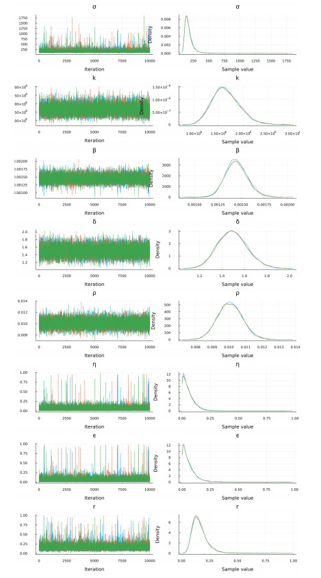
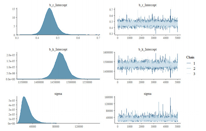
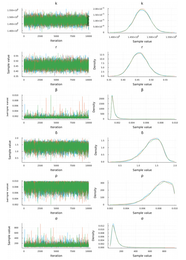
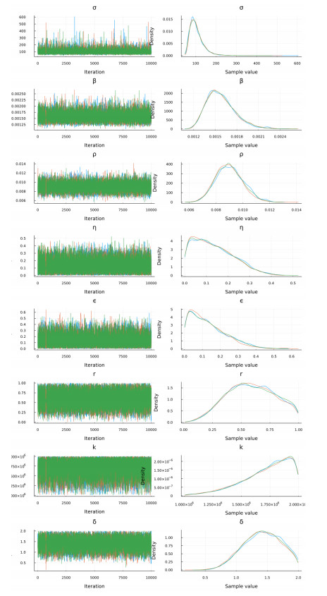
The goal of this work is to estimate the efficacy of interferon therapy in the inhibition of infection by the human immunodeficiency virus type 1 (HIV-1) in a cell culture. For this purpose, three viral dynamics models with the antiviral effect of interferons are presented; the dynamics of cell growth differ among the models, and a variant with Gompertz-type cell dynamics is proposed. A Bayesian statistics approach is used to estimate the cell dynamics parameters, viral dynamics and interferon efficacy. The models are fitted to sets of experimental data on cell growth, HIV-1 infection without interferon therapy and HIV-1 infection with interferon therapy, respectively. The Watanabe-Akaike information criterion (WAIC) is used to determine the model that best fits the experimental data. In addition to the estimated model parameters, the average lifespan of the infected cells and the basic reproductive number are calculated.
- viral dynamics models,
- Bayesian estimation,
- interferon therapy,
- in vitro study,
- model comparison
Citation: Miguel Ángel Rodríguez-Parra, Cruz Vargas-De-León, Flaviano Godinez-Jaimes, Celia Martinez-Lázaro. Bayesian estimation of parameters in viral dynamics models with antiviral effect of interferons in a cell culture[J]. Mathematical Biosciences and Engineering, 2023, 20(6): 11033-11062. doi: 10.3934/mbe.2023488

Related Papers:

Abstract

The goal of this work is to estimate the efficacy of interferon therapy in the inhibition of infection by the human immunodeficiency virus type 1 (HIV-1) in a cell culture. For this purpose, three viral dynamics models with the antiviral effect of interferons are presented; the dynamics of cell growth differ among the models, and a variant with Gompertz-type cell dynamics is proposed. A Bayesian statistics approach is used to estimate the cell dynamics parameters, viral dynamics and interferon efficacy. The models are fitted to sets of experimental data on cell growth, HIV-1 infection without interferon therapy and HIV-1 infection with interferon therapy, respectively. The Watanabe-Akaike information criterion (WAIC) is used to determine the model that best fits the experimental data. In addition to the estimated model parameters, the average lifespan of the infected cells and the basic reproductive number are calculated.

References

[1]	D. D. Ho, A. U. Neumann, A. S. Perelson, W. Chen, J. M. Leonard, M. Markowitz, Rapid turnover of plasma virions and CD4 lymphocytes in HIV-1 infection, Nature, 373 (1995), 123–126.
[2]	A. S. Perelson, A. U. Neumann, M. Markowitz, J. M. Leonard, D. D. Ho, HIV-1 dynamics in vivo: virion clearance rate, infected cells life-span, and viral generation time, Science, 271 (1996), 1582. https://doi.org/10.1126/science.271.5255.1582 doi: 10.1126/science.271.5255.1582
[3]	M. A. Nowak, C. R. Bangham, Population dynamics of immune responses to persistent viruses, Science, 272 (1996), 74–79.
[4]	S. Bonhoeffer, R. M. May, G. M. Shaw, M. A. Nowak, Virus dynamics and drug therapy, Proc. Natl. Acad. Sci. U.S.A., 94 (1997), 6971–6976. https://doi.org/10.1073/pnas.94.13.6971 doi: 10.1073/pnas.94.13.6971
[5]	D. Wodarz, M. A. Nowak, Mathematical models of HIV pathogenesis and treatment, BioEssays, 24 (2002), 1178–1187. https://doi.org/10.1002/bies.10196 doi: 10.1002/bies.10196
[6]	D. S. Callaway, A. S. Perelson, HIV-1 infection and low steady state viral loads, Bull. Math. Biol., 64 (2002), 29–64. https://doi.org/10.1006/bulm.2001.0266 doi: 10.1006/bulm.2001.0266
[7]	A. S. Perelson, Modelling viral and immune system dynamics, Nat. Rev. Immunol., 2 (2002), 28–36. https://doi.org/10.1038/nri700 doi: 10.1038/nri700
[8]	A. U. Neumann, N. P. Lam, H. Dahari, D. R. Gretch, T. E. Wiley, T. J. Layden, et al., Hepatitis C viral dynamics in vivo and the antiviral efficacy of interferon-$\alpha$ therapy, Science, 282 (1998), 103–107.
[9]	H. Dahari, A. Lo, R. M. Ribeiro, A. S. Perelson, Modeling hepatitis C virus dynamics: liver regeneration and critical drug efficacy, J. Theor. Biol., 247 (2007), 371–381. https://doi.org/10.1016/j.jtbi.2007.03.006 doi: 10.1016/j.jtbi.2007.03.006
[10]	P. Baccam, C. Beauchemin, C. A. Macken, F. G. Hayden, A. S. Perelson, Kinetics of influenza A virus infection in humans, J. Virol., 80 (2006), 7590–7599. https://doi.org/10.1128/JVI.01623-05 doi: 10.1128/JVI.01623-05
[11]	C. A. Beauchemin, J. J. McSharry, G. L. Drusano, J. T. Nguyen, G. T. Went, R. M. Ribeiro, et al., Modeling amantadine treatment of influenza A virus in vitro, J. Theor. Biol., 254 (2008), 439–451. https://doi.org/10.1016/j.jtbi.2008.05.031 doi: 10.1016/j.jtbi.2008.05.031
[12]	P. Wu, Z. He, A. Khan, Dynamical analysis and optimal control of an age-since infection HIV model at individuals and population levels, Appl. Math. Modell., 106 (2022), 325–342. https://doi.org/10.1016/j.apm.2022.02.008 doi: 10.1016/j.apm.2022.02.008
[13]	M. Nowak, R. M. May, Virus Dynamics: Mathematical Principles of Immunology and Virology, Oxford University Press, New York, 2000. https://doi.org/10.1038/87836
[14]	D. Dingli, M. D. Cascino, K. Josić, S. J. Russell, Ž. Bajzer, Mathematical modeling of cancer radiovirotherapy, Math. Biosci., 199 (2006), 55–78. https://doi.org/10.1016/j.mbs.2005.11.001 doi: 10.1016/j.mbs.2005.11.001
[15]	H. Ikeda, A. Godinho-Santos, S. Rato, B. Vanwalscappel, F. Clavel, K. Aihara, et al., Quantifying the antiviral effect of IFN on HIV-1 replication in cell culture, Sci. Rep., 5 (2015), 11761. https://doi.org/10.1038/srep11761 doi: 10.1038/srep11761
[16]	P. De Leenheer, H. L. Smith, Virus dynamics: a global analysis, SIAM J. Appl. Math., 63 (2003), 1313–1327. https://doi.org/10.1137/S0036139902406905 doi: 10.1137/S0036139902406905
[17]	A. Korobeinikov, Global properties of basic virus dynamics models, Bull. Math. Biol., 66 (2004), 879–883. https://doi.org/10.1016/j.bulm.2004.02.001 doi: 10.1016/j.bulm.2004.02.001
[18]	A. Gelman, J. B. Carlin, H. S. Stern, D. B. Rubin, Bayesian Data Analysis, Chapman and Hall/CRC, New York, 1995. https://doi.org/10.1201/9780429258411
[19]	C. P. Robert, G. Casella, Introducing Monte Carlo Methods with R, Springer, New York, 2010.
[20]	M. L. Rizzo, Statistical Computing with R, Chapman and Hall/CRC, 2019. https://doi.org/10.1201/9780429192760
[21]	P. C. Burkner, brms: an R package for Bayesian multilevel models using Stan, J. Stat. Software, 80 (2017), 1–28.
[22]	R Core Team, R: A Language and Environment for Statistical Computing, Vienna, Austria, 2020.
[23]	H. Ge, K. Xu, Z. Ghahramani, Turing: a language for flexible probabilistic inference, in International conference on artificial intelligence and statistics, PMLR, (2018), 1682–1690.
[24]	J. Bezanson, A. Edelman, S. Karpinski, V. B. Shah, Julia: A fresh approach to numerical computing, SIAM Rev., 59 (2017), 65–98. https://doi.org/10.1137/141000671 doi: 10.1137/141000671
[25]	M. Plummer, N. Best, K. Cowles, K. Vines, CODA: convergence diagnosis and output analysis for MCMC, R News, 6 (2006), 7–11.
[26]	M. L. Delignette-Muller, C. Dutang, fitdistrplus: an R package for fitting distributions, J. Stat. Software, 64 (2015), 1–34. https://doi.org/10.18637/jss.v064.i04 doi: 10.18637/jss.v064.i04
[27]	P. Van den Driessche, J. Watmough, Reproduction numbers and sub-threshold endemic equilibria for compartmental models of disease transmission, Math. Biosci., 180 (2002), 29–48. https://doi.org/10.1016/S0025-5564(02)00108-6 doi: 10.1016/S0025-5564(02)00108-6
[28]	E. Avila-Vales, N. Chan-Chí, G. E. García-Almeida, C. Vargas-De-León, Stability and Hopf bifurcation in a delayed viral infection model with mitosis transmission, Appl. Math. Comput., 259 (2015), 293–312. https://doi.org/10.1016/j.amc.2015.02.053 doi: 10.1016/j.amc.2015.02.053
[29]	J. D. Meiss, Differential Dynamical Systems, Society for Industrial and Applied Mathematics, Philadelphia, 2007.

Reader Comments

Your name:*

Email:*
© 2023 the Author(s), licensee AIMS Press. This is an open access article distributed under the terms of the Creative Commons Attribution License (http://creativecommons.org/licenses/by/4.0)