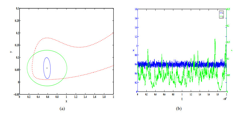
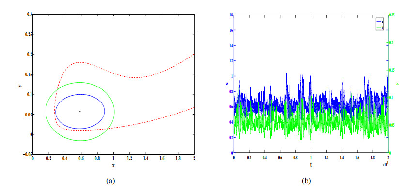
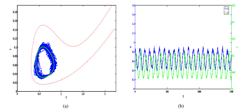
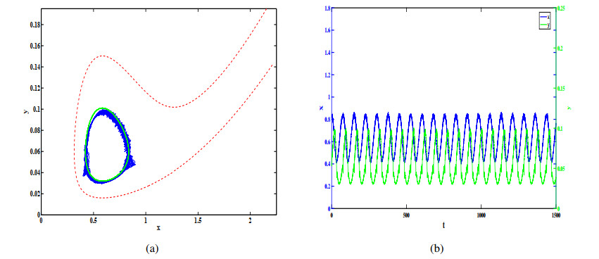
In this study, we investigate a stochastic predator-prey model with anti-predator behavior. We first analyze the noise-induced transition from a coexistence state to the prey-only equilibrium by using the stochastic sensitive function technique. The critical noise intensity for the occurrence of state switching is estimated by constructing confidence ellipses and confidence bands, respectively, for the coexistence the equilibrium and limit cycle. We then study how to suppress the noise-induced transition by using two different feedback control methods to stabilize the biomass at the attraction region of the coexistence equilibrium and the coexistence limit cycle, respectively. Our research indicates that compared with the prey population, the predators appear more vulnerable and prone to extinction in the presence of environmental noise, but it can be prevented by taking some appropriate feedback control strategies.
Citation: Mengya Huang, Anji Yang, Sanling Yuan, Tonghua Zhang. Stochastic sensitivity analysis and feedback control of noise-induced transitions in a predator-prey model with anti-predator behavior[J]. Mathematical Biosciences and Engineering, 2023, 20(2): 4219-4242. doi: 10.3934/mbe.2023197
In this study, we investigate a stochastic predator-prey model with anti-predator behavior. We first analyze the noise-induced transition from a coexistence state to the prey-only equilibrium by using the stochastic sensitive function technique. The critical noise intensity for the occurrence of state switching is estimated by constructing confidence ellipses and confidence bands, respectively, for the coexistence the equilibrium and limit cycle. We then study how to suppress the noise-induced transition by using two different feedback control methods to stabilize the biomass at the attraction region of the coexistence equilibrium and the coexistence limit cycle, respectively. Our research indicates that compared with the prey population, the predators appear more vulnerable and prone to extinction in the presence of environmental noise, but it can be prevented by taking some appropriate feedback control strategies.

| [1] |
B. Dubey, Sajan, A. Kumar, Stability switching and chaos in a multiple delayed prey-predator model with fear effect and anti-predator behavior, Math. Comput. Simul., 188 (2021), 164–192. https://doi.org/10.1016/j.matcom.2021.03.037 doi: 10.1016/j.matcom.2021.03.037

|
| [2] |
Y. Choh, M. Ignacio, M. W. Sabelis, A. Janssen, Predator-prey role reversals, juvenile experience and adult antipredator behaviour, Sci. Rep., 2 (2012), 1–6. https://doi.org/10.1038/srep00728 doi: 10.1038/srep00728
|
| [3] |
G. Polis, C. Myers, R. Holt, The ecology and evolution of intraguild predation: Potential competitors that eat each other, Ann. Rev. Ecol. Syst., 20 (1989), 297–330. https://doi.org/10.1146/annurev.es.20.110189.001501 doi: 10.1146/annurev.es.20.110189.001501
|
| [4] |
S. Kumar, T. Yasuhiro, Dynamics of a predator-prey system with fear and group defense, J. Math. Anal. Appl., 481 (2020), 123471–123494. https://doi.org/10.1016/j.jmaa.2019.123471 doi: 10.1016/j.jmaa.2019.123471
|
| [5] | J. Huang, X. Xia, X. Zhang, S. Ruan, Bifurcation of codimension 3 in a predator-Prey system of leslie type with simplified holling type IV functional response, Int. J. Bifurcation Chaos, 26 (2016). https://doi.org/10.1142/S0218127416500346 |
| [6] |
R. Yang, J. Ma, Analysis of a diffusive predator-prey system with anti-predator behaviour and maturation delay, Chaos Solitons Fractals, 109 (2018), 128–139. https://doi.org/10.1016/j.chaos.2018.02.006 doi: 10.1016/j.chaos.2018.02.006
|
| [7] | C. Li, H. Zhu, Canard cycles for predator-prey systems with Holling types of functional response, J. Differ. Equations, 254 (2013). https://doi.org/10.1016/j.jde.2012.10.003 |
| [8] |
D. Xiao, S. Ruan, Global analysis in a predator-prey system with nonmonotonic functional response, SIAM J. Appl. Math., 61 (2000), 1445–1472. https://doi.org/10.1137/S0036139999361896 doi: 10.1137/S0036139999361896
|
| [9] |
D. Xiao, S. Ruan, Multiple bifurcations in a delayed predator-prey system with nonmonotonic functional response, J. Differ. Equations, 176 (2001), 494–510. https://doi.org/10.1006/jdeq.2000.3982 doi: 10.1006/jdeq.2000.3982
|
| [10] |
H. Zhu, S. A. Campbell, G. S. K. Wolkowicz, Bifurcation analysis of a predator-prey system with nonmonotonic functional response, SIAM J. Appl. Math., 63 (2003), 636–647. https://doi.org/10.1137/S0036139901397285 doi: 10.1137/S0036139901397285
|
| [11] |
B. Tang, Y. Xiao, Bifurcation analysis of a predator-prey model with anti-predator behaviour, Chaos Solitons Fractals, 70 (2015), 58–68. https://doi.org/10.1016/j.chaos.2014.11.008 doi: 10.1016/j.chaos.2014.11.008
|
| [12] |
S. Zhang, S. Yuan, T. Zhang, Dynamic analysis of a stochastic eco-epidemiological model with disease in predators, Stud. Appl. Math., 149 (2021), 5–42. https://doi.org/10.1111/sapm.12489 doi: 10.1111/sapm.12489
|
| [13] | C. Xu, S. Yuan, T. Zhang, Competitive exclusion in a general multi-species chemostat model with stochastic perturbations, Bull. Math. Biol., 83 (2021). https://doi.org/10.1007/s11538-020-00843-7 |
| [14] |
J. Yang, S. Yuan, Dynamics of a toxic producing phytoplankton-zooplankton model with three-dimensional patch, Appl. Math. Lett., 118 (2021), 107146. https://doi.org/10.1016/j.aml.2021.107146 doi: 10.1016/j.aml.2021.107146
|
| [15] |
A. Yang, B. Song, S. Yuan, Noise-induced transitions in a non-smooth SIS epidemic model with media alert, Math. Biosci. Eng., 18 (2020), 745–763. https://doi.org/10.3934/mbe.2021040 doi: 10.3934/mbe.2021040
|
| [16] | Q. Yang, X. Zhang, D. Jiang, M. Shao, Analysis of a stochastic predator-prey model with weak Allee effect and Holling-(n+1) functional response, Commun. Nonlinear Sci. Numer. Simul., 111 (2022). https://doi.org/10.1016/j.cnsns.2022.106454 |
| [17] |
T. Zhang, X. Liu, X. Meng, T. Zhang, Spatio-temporal dynamics near the steady state of a planktonic system, Comput. Math. Appl., 75 (2018), 4490–4504. https://doi.org/10.1016/j.camwa.2018.03.044 doi: 10.1016/j.camwa.2018.03.044
|
| [18] | S. A. Bawa, P. C. Gregg, A. P. Del Socorro, C. Miller, N. R. Andrew, Exposure of Helicoverpa punctigera pupae to extreme temperatures for extended periods negatively impacts on adult population dynamics and reproductive output, J. Therm. Biol., 101 (2021). https://doi.org/10.1016/j.jtherbio.2021.103099 |
| [19] |
C. Kurrer, K. Schulten, Effect of noise and perturbations on limit cycle systems, Phys. D Nonlinear Phenom., 50 (1991), 311–320. https://doi.org/10.1016/0167-2789(91)90001-P doi: 10.1016/0167-2789(91)90001-P
|
| [20] |
F. Gassmann, Noise-induced chaos-order transitions, Phys. Rev. E, 55 (1997), 2215–2221. https://doi.org/10.1103/PhysRevE.55.2215 doi: 10.1103/PhysRevE.55.2215
|
| [21] |
S. Kraut, U. Feudel, Multistability, noise and attractor-hopping: The crucial role of chaotic saddles, Phys. Rev. E, 66 (2002), 015207. https://doi.org/10.1103/PhysRevE.66.015207 doi: 10.1103/PhysRevE.66.015207
|
| [22] | J. B. Gao, S. K. Hwang, J. M. Liu, When can noise induce chaos?, Phys. Rev. Lett., 82 (1999), 1132–1135. https://doi.org/10.1103/PhysRevLett.82.1132 |
| [23] |
Q. Liu, D. Jiang, T. Hayat, A. Alsaedi, Stationary distribution of a regime-switching predator-prey model with anti-predator behaviour and higher-order perturbations, Phys. A, 515 (2019), 199–210. https://doi.org/10.1016/j.physa.2018.09.168 doi: 10.1016/j.physa.2018.09.168
|
| [24] |
S. Zhang, S. Yuan, T. Zhang, A predator-prey model with different response functions to juvenile and adult prey in deterministic and stochastic environments, Appl. Math. Comput., 413 (2022), 126598. https://doi.org/10.1016/j.amc.2021.126598 doi: 10.1016/j.amc.2021.126598
|
| [25] | B. Zhou, B. Han, D. Jiang, T. Hayat, A. Alsaedi, Stationary distribution, extinction and probability density function of a stochastic vegetation-water model in arid ecosystems, J. Nonlinear Sci., 32 (2022). https://doi.org/10.1007/s00332-022-09789-7 |
| [26] | Q. Yang, X. Zhang, D. Jiang, Dynamical behaviors of a stochastic food chain system with ornstein-uhlenbeck process, J. Nonlinear Sci., 32 (2022). https://doi.org/10.1007/s00332-022-09796-8 |
| [27] |
Z. Shi, D. Jiang, X. Zhang, A. Alsaedi, A stochastic SEIRS rabies model with population dispersal: Stationary distribution and probability density function, Appl. Math. Comput., 427 (2022), 427. https://doi.org/10.1016/j.amc.2022.127189 doi: 10.1016/j.amc.2022.127189
|
| [28] | Z. Shi, D. Jiang, Dynamical behaviors of a stochastic HTLV-I infection model with general infection form and ornstein-uhlenbeck process, Chaos Solitons Fractals, 165 (2022). https://doi.org/10.1016/j.chaos.2022.112789 |
| [29] | I. Bashkirtseva, L. Ryashko, I. Tsvetkov, Sensitivity analysis of stochastic equilibria and cycles for the discrete dynamic systems, Dyn. Contin. Discrete Impulsive Syst., 17 (2010), 501–515. |
| [30] |
S. Yuan, D. Wu, G. Lan, H. Wang, Noise-induced transitions in a nonsmooth producer-grazer model with stoichiometric constraints, Bull. Math. Biol., 82 (2020), 1–22. https://doi.org/10.1007/s11538-020-00733-y doi: 10.1007/s11538-020-00733-y
|
| [31] |
L. Ryashko, I. Bashkirtseva, On control of stochastic sensitivity, Autom. Remote Control, 69 (2008), 1171–1180. https://doi.org/10.1134/S0005117908070084 doi: 10.1134/S0005117908070084
|
| [32] |
I. Bashkirtseva, L. Ryashko, Sensitivity and chaos control for the forced nonlinear oscillations, Chaos Solitons Fractals, 26 (2005), 1437–1451. https://doi.org/10.1016/j.chaos.2005.03.029 doi: 10.1016/j.chaos.2005.03.029
|
| [33] |
I. Bashkirtseva, T. Ryazanova, L. Ryashko, Confidence domains in the analysis of noise-induced transition to chaos for Goodwin model of business cycles, Int. J. Bifurcation Chaos, 24 (2014), 1437–1447. https://doi.org/10.1142/S0218127414400203 doi: 10.1142/S0218127414400203
|
Figures(12)

Mengya Huang, Anji Yang, Sanling Yuan, Tonghua Zhang. Stochastic sensitivity analysis and feedback control of noise-induced transitions in a predator-prey model with anti-predator behavior[J]. Mathematical Biosciences and Engineering, 2023, 20(2): 4219-4242. doi: 10.3934/mbe.2023197


 DownLoad: