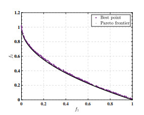
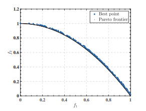
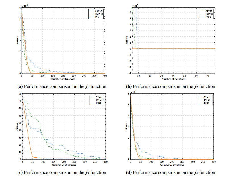
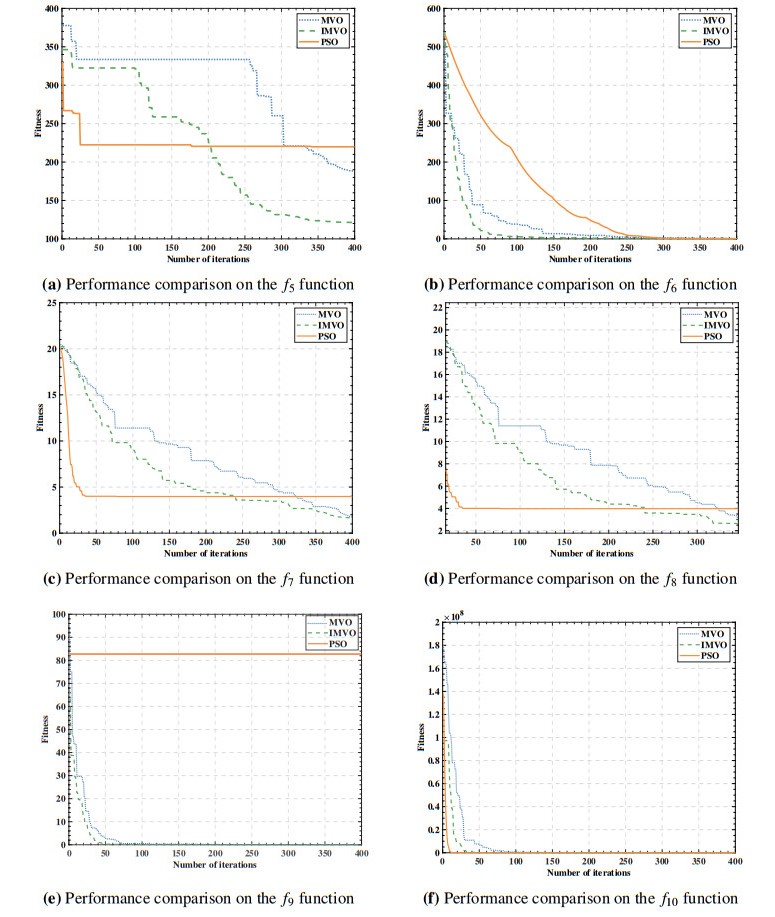
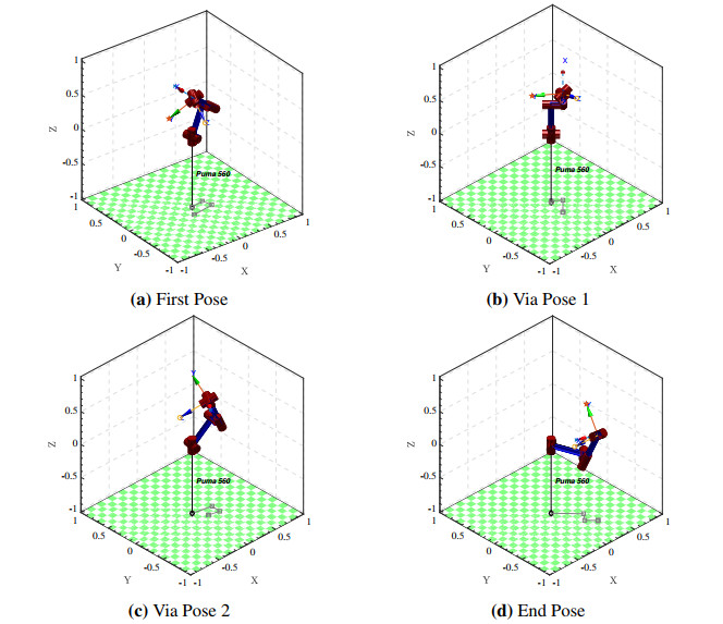
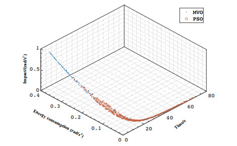
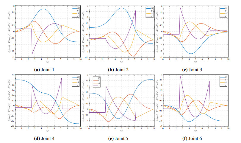
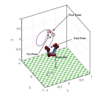
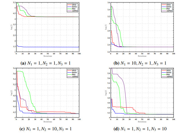
For inefficient trajectory planning of six-degree-of-freedom industrial manipulators, a trajectory planning algorithm based on an improved multiverse algorithm (IMVO) for time, energy, and impact optimization are proposed. The multi-universe algorithm has better robustness and convergence accuracy in solving single-objective constrained optimization problems than other algorithms. In contrast, it has the disadvantage of slow convergence and quickly falls into local optimum. This paper proposes a method to improve the wormhole probability curve, adaptive parameter adjustment, and population mutation fusion to improve the convergence speed and global search capability. In this paper, we modify MVO for multi-objective optimization to derive the Pareto solution set. We then construct the objective function by a weighted approach and optimize it using IMVO. The results show that the algorithm improves the timeliness of the six-degree-of-freedom manipulator trajectory operation within a specific constraint and improves the optimal time, energy consumption, and impact problems in the manipulator trajectory planning.
Citation: Junjie Liu, Hui Wang, Xue Li, Kai Chen, Chaoyu Li. Robotic arm trajectory optimization based on multiverse algorithm[J]. Mathematical Biosciences and Engineering, 2023, 20(2): 2776-2792. doi: 10.3934/mbe.2023130
For inefficient trajectory planning of six-degree-of-freedom industrial manipulators, a trajectory planning algorithm based on an improved multiverse algorithm (IMVO) for time, energy, and impact optimization are proposed. The multi-universe algorithm has better robustness and convergence accuracy in solving single-objective constrained optimization problems than other algorithms. In contrast, it has the disadvantage of slow convergence and quickly falls into local optimum. This paper proposes a method to improve the wormhole probability curve, adaptive parameter adjustment, and population mutation fusion to improve the convergence speed and global search capability. In this paper, we modify MVO for multi-objective optimization to derive the Pareto solution set. We then construct the objective function by a weighted approach and optimize it using IMVO. The results show that the algorithm improves the timeliness of the six-degree-of-freedom manipulator trajectory operation within a specific constraint and improves the optimal time, energy consumption, and impact problems in the manipulator trajectory planning.

| [1] | P. Ngatchou, A. Zarei, A. El-Sharkawi, Pareto multi objective optimization, in Proceedings of the 13th International Conference on, Intelligent Systems Application to Power Systems, (2005), 84–91. https://doi.org/10.1109/ISAP.2005.1599245 |
| [2] | R. Benotsmane, L. Dudás, G. Kovács, Trajectory optimization of industrial robot arms using a newly elaborated "whip-lashing" method, Appl. Sci., 10 (2020). https://doi.org/10.3390/app10238666 |
| [3] |
S. Han, X. Shan, J. Fu, W. Xu, H. Mi, Industrial robot trajectory planning based on improved pso algorithm, J. Phys.: Conf. Ser., 1820 (2021), 012185. https://doi.org/10.1088/1742-6596/1820/1/012185 doi: 10.1088/1742-6596/1820/1/012185

|
| [4] |
X. Peng, G. Chen, Y. Tang, C. Miao, Y. Li, Trajectory optimization of an electro-hydraulic robot, J. Mech. Sci. Technol., 34 (2020), 4281–4294. https://doi.org/10.1007/s12206-020-0919-4 doi: 10.1007/s12206-020-0919-4
|
| [5] | K. Ota, D. K. Jha, T. Oiki, M. Miura, T. Nammoto, D. Nikovski, et al., Trajectory optimization for unknown constrained systems using reinforcement learning, in 2019 IEEE/RSJ International Conference on Intelligent Robots and Systems (IROS), (2019), 3487–3494. https://doi.org/10.1109/IROS40897.2019.8968010 |
| [6] | X. Shi, H. Fang, G. Pi, X. Xu, H. Chen, Time-energy-jerk dynamic optimal trajectory planning for manipulators based on quintic nurbs, in 2018 3rd International Conference on Robotics and Automation Engineering (ICRAE), (2018), 44–49. https://doi.org/10.1109/ICRAE.2018.8586763 |
| [7] |
G. I. Sayed, A. Darwish, A. E. Hassanien, Quantum multiverse optimization algorithm for optimization problems, Neural Comput. Appl., 31 (2019), 2763–2780. https://doi.org/10.1007/s00521-017-3228-9 doi: 10.1007/s00521-017-3228-9
|
| [8] | W. P. Bailón, E. B. Cardiel, I. J. Campos, A. R. Paz, Mechanical energy optimization in trajectory planning for six dof robot manipulators based on eighth-degree polynomial functions and a genetic algorithm, in 2010 7th International Conference on Electrical Engineering Computing Science and Automatic Control, (2010), 446–451. https://doi.org/10.1109/ICEEE.2010.5608583 |
| [9] | S. Lu, Y. Li, Minimum-jerk trajectory planning of a 3-DOF translational parallel manipulator, in 39th Mechanisms and Robotics Conference of International Design Engineering Technical Conferences and Computers and Information in Engineering Conference, 2015. https://doi.org/10.1115/DETC2015-46866 |
| [10] | H. I. Lin, Y. C. Liu, Minimum-jerk robot joint trajectory using particle swarm optimization, in 2011 First International Conference on Robot, Vision and Signal Processing, (2011), 118–121. https://doi.org/10.1109/RVSP.2011.70 |
| [11] | P. Boscariol, A. Gasparetto, R. Vidoni, Planning continuous-jerk trajectories for industrial manipulators, in ASME 2012 11th Biennial Conference on Engineering Systems Design and Analysis, 2012. https://doi.org/10.1115/ESDA2012-82103 |
Figures(9) / Tables(7)

Junjie Liu, Hui Wang, Xue Li, Kai Chen, Chaoyu Li. Robotic arm trajectory optimization based on multiverse algorithm[J]. Mathematical Biosciences and Engineering, 2023, 20(2): 2776-2792. doi: 10.3934/mbe.2023130


 DownLoad: