Stability and Hopf bifurcation of an SIR epidemic model with density-dependent transmission and Allee effect

Xiaofen Lin; Hua Liu; Xiaotao Han; Yumei Wei; Xiaofen Lin; Hua Liu; Xiaotao Han; Yumei Wei

doi:10.3934/mbe.2023129

Mathematical Biosciences and Engineering

2023, Volume 20, Issue 2: 2750-2775. doi: 10.3934/mbe.2023129

Previous Article Next Article

Research article Special Issues

Stability and Hopf bifurcation of an SIR epidemic model with density-dependent transmission and Allee effect

1.
School of Mathematics and Computer Science, Northwest Minzu University, Lanzhou 730030, China
2.
Experimental Teaching Deparment, Northwest Minzu University, Lanzhou 730030, China

Academic Editor: Sanling Yuan

Received: 09 August 2022 Revised: 29 October 2022 Accepted: 13 November 2022 Published: 28 November 2022

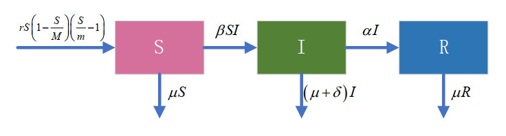
In this paper, an SIR model with a strong Allee effect and density-dependent transmission is proposed, and its characteristic dynamics are investigated. The elementary mathematical characteristic of the model is studied, including positivity, boundedness and the existence of equilibrium. The local asymptotic stability of the equilibrium points is analyzed using linear stability analysis. Our results indicate that the asymptotic dynamics of the model are not only determined using the basic reproduction number ${R_0}$. If ${R_0} < 1$, there are three disease-free equilibrium points, and a disease-free equilibrium is always stable. At the same time, the conditions for other disease-free equilibrium points to be bistable were determined. If ${R_0} > 1$ and in certain conditions, either an endemic equilibrium emerges and is locally asymptotically stable, or the endemic equilibrium becomes unstable. What must be emphasized is that there is a locally asymptotically stable limit cycle when the latter happens. The Hopf bifurcation of the model is also discussed using topological normal forms. The stable limit cycle can be interpreted in a biological significance as a recurrence of the disease. Numerical simulations are used to verify the theoretical analysis. Taking into account both density-dependent transmission of infectious diseases and the Allee effect, the dynamic behavior becomes more interesting than when considering only one of them in the model. The Allee effect makes the SIR epidemic model bistable, which also makes the disappearance of diseases possible, since the disease-free equilibrium in the model is locally asymptotically stable. At the same time, persistent oscillations due to the synergistic effect of density-dependent transmission and the Allee effect may explain the recurrence and disappearance of disease.
- strong Allee effect,
- density-dependent transmission,
- SIR epidemic model,
- bistability,
- Hopf bifurcation
Citation: Xiaofen Lin, Hua Liu, Xiaotao Han, Yumei Wei. Stability and Hopf bifurcation of an SIR epidemic model with density-dependent transmission and Allee effect[J]. Mathematical Biosciences and Engineering, 2023, 20(2): 2750-2775. doi: 10.3934/mbe.2023129

Related Papers:

Abstract

In this paper, an SIR model with a strong Allee effect and density-dependent transmission is proposed, and its characteristic dynamics are investigated. The elementary mathematical characteristic of the model is studied, including positivity, boundedness and the existence of equilibrium. The local asymptotic stability of the equilibrium points is analyzed using linear stability analysis. Our results indicate that the asymptotic dynamics of the model are not only determined using the basic reproduction number ${R_0}$. If ${R_0} < 1$, there are three disease-free equilibrium points, and a disease-free equilibrium is always stable. At the same time, the conditions for other disease-free equilibrium points to be bistable were determined. If ${R_0} > 1$ and in certain conditions, either an endemic equilibrium emerges and is locally asymptotically stable, or the endemic equilibrium becomes unstable. What must be emphasized is that there is a locally asymptotically stable limit cycle when the latter happens. The Hopf bifurcation of the model is also discussed using topological normal forms. The stable limit cycle can be interpreted in a biological significance as a recurrence of the disease. Numerical simulations are used to verify the theoretical analysis. Taking into account both density-dependent transmission of infectious diseases and the Allee effect, the dynamic behavior becomes more interesting than when considering only one of them in the model. The Allee effect makes the SIR epidemic model bistable, which also makes the disappearance of diseases possible, since the disease-free equilibrium in the model is locally asymptotically stable. At the same time, persistent oscillations due to the synergistic effect of density-dependent transmission and the Allee effect may explain the recurrence and disappearance of disease.

References

[1]	R. M. Anderson, R. M. May, Population biology of infectious diseases, Nature, 280 (1979), 361–367. https://doi.org/10.1007/978-3-642-68635-1 doi: 10.1007/978-3-642-68635-1
[2]	P. Daszak, L. Berger, A. A. Cunningham, A. D. Hyatt, D. E. Green, R. Speare, Emerging infectious diseases and amphibian population declines, Emerg. Infect. Dis., 5 (1999), 735–748. https://doi.org/10.3201/eid0506.990601 doi: 10.3201/eid0506.990601
[3]	F. D. Castro, B. Bolker, Mechanisms of disease-induced extinction, Ecol. Lett., 8 (2005), 117–126. https://doi.org/10.1111/j.1461-0248.2004.00693.x doi: 10.1111/j.1461-0248.2004.00693.x
[4]	D. T. Haydon, M. K. Laurenson, C. Sillero-Zubiri, Integrating epidemiology into population viability analysis: managing the risk posed by rabies and canine distemper to the Ethiopian wolf, Conserv. Biol., 16 (2002), 1372–1385. https://doi.org/10.1046/j.1523-1739.2002.00559.x doi: 10.1046/j.1523-1739.2002.00559.x
[5]	F. M. Hilker, M. Langlais, S. V. Petrovskii, H. Malchow, A diffusive SI model with Allee effect and application to FIV, Math. Biosci, 206 (2007), 61–80. https://doi.org/10.1016/j.mbs.2005.10.003 doi: 10.1016/j.mbs.2005.10.003
[6]	F. M. Hilker, M. A. Lewis, H. Seno, M. Langlais, H. Malchow, Pathogens can slow down or reverse invasion fronts of their hosts, Biol. Invasions, 7 (2005), 817–832. https://doi.org/10.1007/s10530-005-5215-9 doi: 10.1007/s10530-005-5215-9
[7]	P. J. Hudson, A. P. Rizzoli, B. T. Grenfell, The Ecology of Wildlife Diseases, Oxford University Press, Oxford, 2001, 45–62.
[8]	J. Y. Zhou, Y. Zhao, Y. Ye, Y. X. Bao, Bifurcation analysis of a fractional-order simplicial sirs system induced by double delays, Int. J. Bifurcat. Chaos, 32 (2022), 2250068. https://doi.org/10.1142/S0218127422500687 doi: 10.1142/S0218127422500687
[9]	M. Begon, M. Bennett, R. G. Bowers, N. P. French, S. M. Hazel, J. Turner, A clarification of transmission terms in host-microparasite models: Numbers, densities and areas, Epidemiol. Infect., 129 (2002), 147–153. https://doi.org/10.1017/s0950268802007148 doi: 10.1017/s0950268802007148
[10]	J. S. Zhou, H. W. Hethcote, Population size dependent incidence in models for diseases without immunity, J. Math. Biol., 32 (1994), 809–834. https://doi.org/10.1007/bf00168799
[11]	F. M. Hilker, M. Langlais, H. Malchow, The Allee effect and infectious diseases: extinction, multistability and the (dis-)appearance of oscillations, Am. Nat., 173 (2009), 72–88. https://doi.org/10.1086/593357 doi: 10.1086/593357
[12]	W. C. Allee, Animal Aggregation: A Study in General Sociology, University of Chicago Press, Chicago, 1931. https://doi.org/10.5962/bhl.title.7313
[13]	S. H. Liu, S. G. Ruan, X. N. Zhang, Nonlinear dynamics of avian influenza epidemic models, Math. Biosci., 283 (2017), 118–135. https://doi.org/10.1016/j.mbs.2016.11.014 doi: 10.1016/j.mbs.2016.11.014
[14]	B. Dennis, Allee effects: Population growth, critical density and the chance of extinction, Nat. Resour. Model, 3 (1989), 481–538. https://doi.org/10.1111/j.1939-7445.1989.tb00119.x doi: 10.1111/j.1939-7445.1989.tb00119.x
[15]	F. Courchamp, T. Clutton-Brock, B. Grenfell, F. Courchamp, T. Clutton-Brock, B. Grenfell, et al., Inverse density dependence and the Allee effect, Trends Ecol. Evolut, 14 (1999), 405–410. https://doi.org/10.1016/s0169-5347(99)01683-3 doi: 10.1016/s0169-5347(99)01683-3
[16]	P. A. Stephens, W. J. Sutherland, R. P. Freckleton, What is the Allee effect?, Oikos, 87 (1999), 185–190. https://doi.org/10.2307/3547011 doi: 10.2307/3547011
[17]	P. A. Stephens, W. J. Sutherland, Consequences of the Allee effect for behaviour, ecology and conservation, Trends Ecol. Evolut., 14 (1999), 401–405. https://doi.org/10.1016/s0169-5347(99)01684-5 doi: 10.1016/s0169-5347(99)01684-5
[18]	A. Y. Morozov, M. Banerjee, S. V. Petrovskii, Long-term transients and complex dynamics of a stage-structured population with time delay and the Allee effect, J. Theor. Biol., 396 (2016), 116–124. https://doi.org/10.1016/j.jtbi.2016.02.016 doi: 10.1016/j.jtbi.2016.02.016
[19]	S. Biswas, M. D. Saifuddin, S. K. Sasmal, S. Samanta, N. Pal, F. Ababneh, et al., A delayed preypredator system with prey subject to the strong Allee effect and disease, Nonlinear. Dynam., 84 (2016), 1569–1594. https://doi.org/10.1007/s11071-015-2589-9 doi: 10.1007/s11071-015-2589-9
[20]	S. V. Petrovskii, A. Y. Morozov, E. Venturino, Allee effect makes possible patchy invasion in a predator-prey system, Ecol. Lett., 5 (2010), 345–352. https://doi.org/10.1046/j.1461-0248.2002.00324.x doi: 10.1046/j.1461-0248.2002.00324.x
[21]	L. Shi, H. Liu, Y. M. Wei, M. Ma, Y. Ye, The permanence and periodic solution of a competitive system with infinite delay, feedback control, and Allee effect, Adv. Differ. Equation, 2018 (2018), 1–14. https://doi.org/10.1186/s13662-018-1860-z doi: 10.1186/s13662-018-1860-z
[22]	Y. Ye, H. Liu, Y. M. Wei, M. Ma, K. Zhang, Dynamic study of a predator-prey model with weak Allee effect and delay, Adv. Math. Phys., 2019 (2019). https://doi.org/10.1155/2019/7296461 doi: 10.1155/2019/7296461
[23]	S. K. Sasmal, Population dynamics with multiple Allee effects induced by fear factors-a mathematical study on prey-predator interactions, Appl. Math. Model., 64 (2018), 1–14. https://doi.org/10.1016/j.apm.2018.07.021 doi: 10.1016/j.apm.2018.07.021
[24]	M. Sen, M. Banerjee, Y. Takeuchi, Influence of Allee effect in prey populations on the dynamics of two-prey-one-predator model, Math. Biosci. Eng., 15 (2018), 883–904. https://doi.org/10.3934/mbe.2018040 doi: 10.3934/mbe.2018040
[25]	Y. L. Cai, C. D. Zhao, W. M. Wang, J. F. Wang, Dynamics of a Leslie-Gower predator-prey model with additive Allee effect, Appl. Math. Model., 39 (2015), 2092–2106. https://doi.org/10.1016/j.apm.2014.09.038 doi: 10.1016/j.apm.2014.09.038
[26]	R. J. Han, B. X. Dai, Spatiotemporal pattern formation and selection induced by nonlinear cross-diffusion in a toxic-phytoplankton-zooplankton model with Allee effect, Nonlinear Anal. Real., 45 (2018) 822–853. https://doi.org/10.1016/j.nonrwa.2018.05.018 doi: 10.1016/j.nonrwa.2018.05.018
[27]	M. Banerjee, Y. Takeuchi, Maturation delay for the predators can enhance stable coexistence for a class of prey-predator models, J. Theor. Biol., 412 (2017) 154–171. https://doi.org/10.1016/j.jtbi.2016.10.016. doi: 10.1016/j.jtbi.2016.10.016
[28]	Y. Ye, Y. Zhao, Bifurcation analysis of a delay-induced predator–prey model with Allee effect and prey group defense, Int. J. Bifurcat. Chaos, 31 (2021), 2150158. https://doi.org/10.1142/S0218127421501583 doi: 10.1142/S0218127421501583
[29]	A. Deredec, F. Courchamp, Combined impacts of Allee effects and parasitism. Oikos, 112 (2006), 667–679. https://doi.org/10.1111/j.0030-1299.2006.14243.x doi: 10.1111/j.0030-1299.2006.14243.x
[30]	A. Friedman, A. A. Yakubu, Fatal disease and demographic Allee effect: population persistence and extinction. J. Biol. Dyn., 6 (2012), 495–508. https://doi.org/10.1080/17513758.2011.630489 doi: 10.1080/17513758.2011.630489
[31]	H. R. Thieme, T. Dhirasakdanon, Z. Han, R. Trevino, Species decline and extinction: synergy of infectious diseases and Allee effect?, J. Biol. Dyn., 3 (2009), 305–323. https://doi.org/10.1080/17513750802376313 doi: 10.1080/17513750802376313
[32]	R. Burrows, H. Hofer, M. L. East, Population dynamics, intervention and survival in African wild dogs (Lycaon pictus), Proc. R. Soc. Lond. B, 262 (1995), 235–245. https://doi.org/10.1098/rspb.1995.0201 doi: 10.1098/rspb.1995.0201
[33]	F. Courchamp, T. Clutton-Brock, B. Grenfell, Multipack dynamics and the Allee effect in the African wild dog, Lycaon pictus, Anim. Conserv., 3 (2000), 277–285. https://doi.org/10.1111/j.1469-1795.2000.tb00113.x doi: 10.1111/j.1469-1795.2000.tb00113.x
[34]	D. L. Clifford, J. A. K. Mazet, E. J. Dubovi, D. K. Garcelon, T. J. Coonan, P. A. Conrad, et al., Pathogen exposure in endangered island fox (Urocyon littoralis) populations: implications for conservation management, Biol. Conserv., 131 (2006), 230–243. https://doi.org/10.1016/j.biocon.2006.04.029 doi: 10.1016/j.biocon.2006.04.029
[35]	E. Angulo, G. W. Roemer, L. Berec, J. Gascoigne, F. Courchamp, Double Allee effects and extinction in the island fox, Conserv. Biol., 21 (2007), 1082–1091. https://doi.org/10.1111/j.1523-1739.2007.00721.x doi: 10.1111/j.1523-1739.2007.00721.x
[36]	L. J. Rachowicz, J. M. Hero, R. A. Alford, J. W. Taylor, J. A. T. Morgan, V. T. Vredenburg, et. al., The novel and endemic pathogen hypotheses: competing explanations for the origin of emerging infectious diseases of wildlife, Conserv. Biol., 19 (2005), 1441–1448. https://doi.org/10.1111/j.1523-1739.2005.00255.x doi: 10.1111/j.1523-1739.2005.00255.x
[37]	L. J. Rachowicz, R. A. Knapp, J. A. T. Morgan, M. J. Stice, V. T. Vredenburg, J. M. Parker, et al., Emerging infectious disease as a proximate cause of amphibian mass mortality, Ecology, 87 (2006), 1671–1683. https://doi.org/10.1890/0012-9658(2006)87[1671:eidaap]2.0.co;2 doi: 10.1890/0012-9658(2006)87[1671:eidaap]2.0.co;2
[38]	L. F. Skerrat, L. Berger, R. Speare, S. Cashins, K. R. McDonald, A. D. Phillott, et al., Spread of chytridiomycosis has caused the rapid global decline and extinction of frogs, EcoHealth, 4 (2007), 125–134. https://doi.org/10.1007/s10393-007-0093-5 doi: 10.1007/s10393-007-0093-5
[39]	Y. Kang, C. Castillo-Chavez, A simple epidemiological model for populations in the wild with Allee effects and disease-modified fitness, Discrete Contin. Dyn. Syst. B, 19 (2014), 89–130. https://doi.org/10.1090/conm/618/12342 doi: 10.1090/conm/618/12342
[40]	J. M. Drake, Allee effects and the risk of biological invasion, Risk Anal., 24 (2004), 795–802. https://doi.org/10.1111/j.0272-4332.2004.00479.x doi: 10.1111/j.0272-4332.2004.00479.x
[41]	Y. Y. Lv, L. J. Chen, F. D. Chen, Z. Li, Stability and bifurcation in an SI epidemic model with additive Allee effect and time delay, Int. J. Bifurcat. Chaos, 31 (2021), 2150060. https://doi.org/10.1142/S0218127421500607 doi: 10.1142/S0218127421500607
[42]	W. Q. Yin, Z. Li, F. D. Chen, M. X. He, Modeling Allee effect in the Leslie-Gower predator-prey system incorporating a prey refuge, Int. J. Bifurcat. Chaos, 32 (2022), 2250086. https://doi.org/10.1142/S0218127422500869 doi: 10.1142/S0218127422500869
[43]	Y. Y. Lv, L. J. Chen, F. D. Chen, Stability and bifurcation in a single species logistic model with additive Allee effect and feedback control, Adv. Differ. Equation, 2020 (2020). https://doi.org/10.1186/s13662-020-02586-0 doi: 10.1186/s13662-020-02586-0
[44]	K. Fang, Z. L. Zhu, F. D. Chen, Z. Li, Qualitative and bifurcation analysis in a leslie-gower model with Allee effect, Qual. Theory Dyn. Syst., 21 (2022). https://doi.org/10.1007/s12346-022-00591-0 doi: 10.1007/s12346-022-00591-0
[45]	F. D. Chen, X. Y. Guan, X. Y. Huang, H. Deng, Dynamic behaviors of a Lotka-Volterra type predator-prey system with Allee effect on the predator species and density dependent birth rate on the prey species, Open Math., 17 (2019), 1186–1202. https://doi.org/10.1515/math-2019-0082 doi: 10.1515/math-2019-0082
[46]	Y. Kang, C. Castillo-Chavez, Dynamics of SI models with both horizontal and vertical transmissions as well as Allee effects, Math. Biosci. 248 (2014), 97–116. https://doi.org/10.1016/j.mbs.2013.12.006 doi: 10.1016/j.mbs.2013.12.006
[47]	F. M. Hilker, Epidemiological models with demographic Allee effect, Biomat, 2008 (2009), 52–77. https://doi.org/10.1142/9789814271820_0003 doi: 10.1142/9789814271820_0003
[48]	Y. A. Kuznetsov, Elements of Applied Bifurcation Theory, 2nd edition, Springer New York, New York, 2004. https://doi.org/10.1007/978-1-4757-3978-7
[49]	H. Liu, K. Zhang, Y. Ye, Y. M. Wei, M. Ma, Dynamic complexity and bifurcation analysis of a host-parasitoid model with Allee effect and Holling type III functional response, Adv. Differ. Equation, 507 (2019). https://doi.org/10.1186/s13662-019-2430-8 doi: 10.1186/s13662-019-2430-8
[50]	Z. F. Zhang, T. R. Ding, W. Z. Huang, Z. X. Dong, Qualitative Theory of Differential Equation, Science Press, Beijing, 1992.

Reader Comments

Your name:*

Email:*
© 2023 the Author(s), licensee AIMS Press. This is an open access article distributed under the terms of the Creative Commons Attribution License (http://creativecommons.org/licenses/by/4.0)