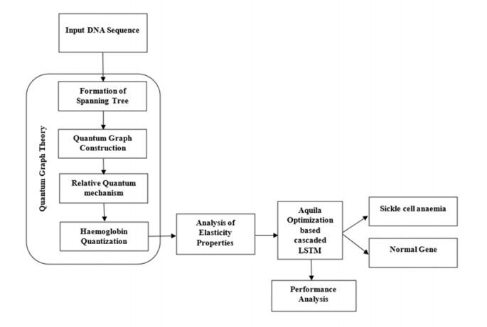
Recently genetic disorders are the most common reason for human fatality. Sickle Cell anemia is a monogenic disorder caused by A-to-T point mutations in the β-globin gene which produces abnormal hemoglobin S (Hgb S) that polymerizes at the state of deoxygenation thus resulting in the physical deformation or erythrocytes sickling. This shortens the expectancy of human life. Thus, the early diagnosis and identification of sickle cell will aid the people in recognizing signs and to take treatments. The manual identification is a time consuming one and might outcome in the misclassification of count as there is millions of red blood cells in one spell. So as to overcome this, data mining approaches like Quantum graph theory model and classifier is effective in detecting sickle cell anemia with high precision rate. The proposed work aims at presenting a mathematical modeling using Quantum graph theory to extract elasticity properties and to distinguish them as normal cells and sickle cell anemia (SCA) in red blood cells. Initially, input DNA sequence is taken and the elasticity property features are extracted by using Quantum graph theory model at which the formation of spanning tree is made followed by graph construction and Hemoglobin quantization. After which, the extracted properties are optimized using Aquila optimization and classified using cascaded Long Short-Term memory (LSTM) to attain the classified outcome of sickle cell and normal cells. Finally, the performance assessment is made and the outcomes attained in terms of accuracy, precision, sensitivity, specificity, and AUC are compared with existing classifier to validate the proposed system effectiveness.
Citation: P. Balamanikandan, S. Jeya Bharathi. A mathematical modelling to detect sickle cell anemia using Quantum graph theory and Aquila optimization classifier[J]. Mathematical Biosciences and Engineering, 2022, 19(10): 10060-10077. doi: 10.3934/mbe.2022470
Recently genetic disorders are the most common reason for human fatality. Sickle Cell anemia is a monogenic disorder caused by A-to-T point mutations in the β-globin gene which produces abnormal hemoglobin S (Hgb S) that polymerizes at the state of deoxygenation thus resulting in the physical deformation or erythrocytes sickling. This shortens the expectancy of human life. Thus, the early diagnosis and identification of sickle cell will aid the people in recognizing signs and to take treatments. The manual identification is a time consuming one and might outcome in the misclassification of count as there is millions of red blood cells in one spell. So as to overcome this, data mining approaches like Quantum graph theory model and classifier is effective in detecting sickle cell anemia with high precision rate. The proposed work aims at presenting a mathematical modeling using Quantum graph theory to extract elasticity properties and to distinguish them as normal cells and sickle cell anemia (SCA) in red blood cells. Initially, input DNA sequence is taken and the elasticity property features are extracted by using Quantum graph theory model at which the formation of spanning tree is made followed by graph construction and Hemoglobin quantization. After which, the extracted properties are optimized using Aquila optimization and classified using cascaded Long Short-Term memory (LSTM) to attain the classified outcome of sickle cell and normal cells. Finally, the performance assessment is made and the outcomes attained in terms of accuracy, precision, sensitivity, specificity, and AUC are compared with existing classifier to validate the proposed system effectiveness.

| [1] |
M. C. V. Schie, S. Jainandunsing, J. E. R. Lennep, Monogenetic disorders of the cholesterol metabolism and premature cardiovascular disease, Eur. J. Pharmacol., 816 (2017), 146–153. https://doi.org/10.1016/j.ejphar.2017.09.046 doi: 10.1016/j.ejphar.2017.09.046

|
| [2] |
J. Zhou, Q. Lu, R. Xu, L. Gui, H. Wang, EL_LSTM: prediction of DNA-binding residue from protein sequence by combining long short-term memory and ensemble learning, IEEE/ACM Trans. Comput. Biol. Bioinf., 17 (2018), 124–135. https://doi.org/10.1109/TCBB.2018.2858806 doi: 10.1109/TCBB.2018.2858806
|
| [3] |
Q. Zhang, P. Liu, X. Wang, Y. Zhang, Y. Han, B. Yu, StackPDB: predicting DNA-binding proteins based on XGB-RFE feature optimization and stacked ensemble classifier, Appl. Soft Comput., 99 (2021), 106921. https://doi.org/10.1016/j.asoc.2020.106921 doi: 10.1016/j.asoc.2020.106921
|
| [4] |
S. Demirci, N. Uchida, J. F. Tisdale, Gene therapy for sickle cell disease: An update, Cytotherapy, 20 (2018), 899–910. https://doi.org/10.1016/j.jcyt.2018.04.003 doi: 10.1016/j.jcyt.2018.04.003
|
| [5] |
V. M. Pinto, M. Balocco, S. Quintino, G. L. Forni, Sickle cell disease: A review for the internist, Int. Emerg. Med., 14 (2019), 1051–1064. https://doi.org/10.1007/s11739-019-02160-x doi: 10.1007/s11739-019-02160-x
|
| [6] |
X. Yang, Q. Zhou, W. Zhou, M. Zhong, X. Guo, X. Wang, et al., A cell‐free DNA barcode‐enabled single‐molecule test for noninvasive prenatal diagnosis of monogenic disorders: Application to β‐thalassemia, Adv. Sci., 6 (2019), 1802332. https://doi.org/10.1002/advs.201802332 doi: 10.1002/advs.201802332
|
| [7] |
C. M. Dasari, R. Bhukya, Explainable deep neural networks for novel viral genome prediction, Appl. Intell., 52(2022), 3002–3017. https://doi.org/10.1007/s10489-021-02572-3 doi: 10.1007/s10489-021-02572-3
|
| [8] |
J. T. Shieh, M. Penon-Portmann, K. H. Wong, M. Levy-Sakin, M. Verghese, A. Slavotinek, et al., Application of full-genome analysis to diagnose rare monogenic disorders, NPJ Genomic Med., 6 (2021), 1–10. https://doi.org/10.1038/s41525-021-00241-5 doi: 10.1038/s41525-021-00241-5
|
| [9] |
S. Mettananda, D. R. Higgs, Molecular basis and genetic modifiers of thalassemia, Hematol. Oncol. Clin., 32(2018), 177–191. https://doi.org/10.1016/j.hoc.2017.11.003 doi: 10.1016/j.hoc.2017.11.003
|
| [10] | B. Chakraborty, Genetic algorithm with fuzzy fitness function for feature selection. In Industrial Electronics, 2002. ISIE 2002. Proceedings of the 2002 IEEE International Symposium on, 1 (2002), 315–319. https://doi.org/10.1109/ISIE.2002.1026085 |
| [11] |
D. Singh, S. P. Singh, Self-organization and learning methods in short term electric load forecasting: A review, Electr. Power Compon. Syst., 30 (2002), 1075–1089. https://doi.org/10.1080/15325000290085370 doi: 10.1080/15325000290085370
|
| [12] |
E. C. Morabito, M. Versaci, A fuzzy neural approach to localizing holes in conducting plates, IEEE Trans. Magn., 37 (2001), 3534–3537. https://doi.org/10.1109/20.952655 doi: 10.1109/20.952655
|
| [13] |
L. Abualigah, A. Diabat, S. Mirjalili, M. Abd Elaziz, A. H. Gandomi, The arithmetic optimization algorithm, Comput. Methods Appl. Mech. Eng., 376 (2021), 113609. https://doi.org/10.1016/j.cma.2020.113609 doi: 10.1016/j.cma.2020.113609
|
| [14] |
J. O. Agushaka, A. E. Ezugwu, L. Abualigah, Dwarf mongoose optimization algorithm, Comput. Methods Appl. Mech. Eng., 391 (2022), 114570. https://doi.org/10.1016/j.cma.2022.114570 doi: 10.1016/j.cma.2022.114570
|
| [15] |
L. Abualigah, M. Abd Elaziz, P. Sumari, Z. W. Geem, A. H. Gandomi, Reptile Search Algorithm (RSA): A nature-inspired meta-heuristic optimizer, Exp. Syst. Appl., 191 (2022), 116158. https://doi.org/10.1016/j.eswa.2021.116158 doi: 10.1016/j.eswa.2021.116158
|
| [16] |
O. N. Oyelade, A. E. S. Ezugwu, T. I. Mohamed, L. Abualigah, Ebola optimization search algorithm: A new nature-inspired metaheuristic optimization algorithm, IEEE Access, 10 (2022), 16150–16177. https://doi.org/10.1109/ACCESS.2022.3147821 doi: 10.1109/ACCESS.2022.3147821
|
| [17] |
L. Abualigah, D. Yousri, M. Abd Elaziz, A. A. Ewees, M. A. Al-Qaness, A. H. Gandomi, Aquila optimizer: a novel meta-heuristic optimization algorithm, Comput. Ind. Eng., 157 (2021), 107250. https://doi.org/10.1016/j.cie.2021.107250 doi: 10.1016/j.cie.2021.107250
|
| [18] |
J. A. López-Rivera, E. Pérez-Palma, J. Symonds, A. S. Lindy, D. A. McKnight, C. Leu, et al., A catalogue of new incidence estimates of monogenic neurodevelopmental disorders caused by de novo variants, Brain, 143(2020), 1099–1105. https://doi.org/10.1093/brain/awaa051 doi: 10.1093/brain/awaa051
|
| [19] |
E. K. L. Chiu, W. W. I. Hui, R. W. K. Chiu, cfDNA screening and diagnosis of monogenic disorders–where are we heading, Prenatal Diagn., 38 (2018), 52–58. https://doi.org/10.1002/pd.5207 doi: 10.1002/pd.5207
|
| [20] |
A. M. Quinn, B. N. Valcarcel, M. M. Makhamreh, H. B. Al-Kouatly, S. I. Berger, A systematic review of monogenic etiologies of nonimmune hydrops fetalis, Genet. Med., 23 (2021), 3–12. https://doi.org/10.1038/s41436-020-00967-0 doi: 10.1038/s41436-020-00967-0
|
| [21] |
M. E. Niemi, H. C. Martin, D. L. Rice, G. Gallone, S. Gordon, M. Kelemen, et al., Common genetic variants contribute to risk of rare severe neurodevelopmental disorders, Nature, 562 (2018), 268–271. https://doi.org/10.1038/s41586-018-0566-4 doi: 10.1038/s41586-018-0566-4
|
| [22] |
M. Zech, R. Jech, S. Boesch, M. Škorvánek, S. Weber, M. Wagner, et al., Monogenic variants in dystonia: an exome-wide sequencing study, Lancet Neurol., 19 (2020), 908–918. https://doi.org/10.1016/S1474-4422(20)30312-4 doi: 10.1016/S1474-4422(20)30312-4
|
| [23] |
D. M. Connaughton, C. Kennedy, S. Shril, N. Mann, S. L. Murray, P. A. Williams, et al., Monogenic causes of chronic kidney disease in adults, Kidney Int., 95 (2019), 914–928. https://doi.org/10.1016/j.kint.2018.10.031 doi: 10.1016/j.kint.2018.10.031
|
| [24] |
G. Valles-Ibáñez, A. Esteve-Sole, M. Piquer, E. A. González-Navarro, J. Hernandez-Rodriguez, H. Laayouni, et al., Evaluating the genetics of common variable immunodeficiency: monogenetic model and beyond, Front. Immunol., 9 (2018), 636. https://doi.org/10.3389/fimmu.2018.00636 doi: 10.3389/fimmu.2018.00636
|
| [25] |
J. M. Alperin, L. Ortiz-Fernández, A. H. Sawalha, Monogenic lupus: a developing paradigm of disease, Front. Immunol., 9 (2018), 2496. https://doi.org/10.3389/fimmu.2018.02496 doi: 10.3389/fimmu.2018.02496
|
| [26] |
J. J. Ashton, E. Mossotto, I. S. Stafford, R. Haggarty, T. A. Coelho, A. Batra, et al., Genetic sequencing of pediatric patients identifies mutations in monogenic inflammatory bowel disease genes that translate to distinct clinical phenotypes, Clin. Transl. Gastroenterol., 11 (2020). https://doi.org/10.14309/ctg.0000000000000129 doi: 10.14309/ctg.0000000000000129
|
| [27] |
J. C. Almlöf, S. Nystedt, D. Leonard, M. L. Eloranta, G. Grosso, C. Sjöwall, et al., Whole-genome sequencing identifies complex contributions to genetic risk by variants in genes causing monogenic systemic lupus erythematosus, Hum. Genet., 138 (2019), 141–150. https://doi.org/10.1007/s00439-018-01966-7 doi: 10.1007/s00439-018-01966-7
|
| [28] |
S. Vidal, N. Brandi, P. Pacheco, J. Maynou, G. Fernandez, C. Xiol, et al., The most recurrent monogenic disorders that overlap with the phenotype of Rett syndrome, Eur. J. Paediatr. Neurol., 23 (2019), 609–620. https://doi.org/10.1016/j.ejpn.2019.04.006 doi: 10.1016/j.ejpn.2019.04.006
|
| [29] |
S. Butscheidt, A. Delsmann, T. Rolvien, F. Barvencik, M. Al-Bughaili, S. Mundlos, et al., Mutational analysis uncovers monogenic bone disorders in women with pregnancy-associated osteoporosis: three novel mutations in LRP5, COL1A1, and COL1A2, Osteoporosis Int., 29 (2018), 1643–1651. https://doi.org/10.1007/s00198-018-4499-4 doi: 10.1007/s00198-018-4499-4
|
| [30] |
F. Cerrato, A. Sparago, F. Ariani, F. Brugnoletti, L. Calzari, F. Coppedè, et al., DNA methylation in the diagnosis of monogenic diseases, Genes, 11 (2020), 355. https://doi.org/10.3390/genes11040355 doi: 10.3390/genes11040355
|
| [31] |
S. Yeruva, M. S. Varalakshmi, B. P. Gowtham, Y. H. Chandana, P. K. Prasad, Identification of sickle cell anemia using deep neural networks, Emerging Sci. J., 5 (2021), 200–210. https://doi.org/10.28991/esj-2021-01270 doi: 10.28991/esj-2021-01270
|
Figures(9) / Tables(1)

P. Balamanikandan, S. Jeya Bharathi. A mathematical modelling to detect sickle cell anemia using Quantum graph theory and Aquila optimization classifier[J]. Mathematical Biosciences and Engineering, 2022, 19(10): 10060-10077. doi: 10.3934/mbe.2022470


 DownLoad: