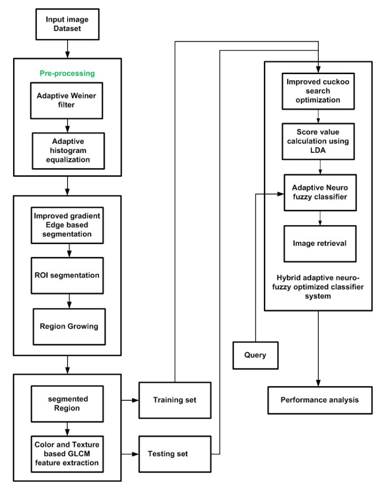
The quantity of scientific images associated with patient care has increased markedly in recent years due to the rapid development of hospitals and research facilities. Every hospital generates more medical photographs, resulting in more than 10 GB of data per day being produced by a single image appliance. Software is used extensively to scan and locate diagnostic photographs to identify patient's precise information, which can be valuable for medical science research and advancement. An image recovery system is used to meet this need. This paper suggests an optimized classifier framework focused on a hybrid adaptive neuro-fuzzy approach to accomplish this goal. In the user query, similarity measurement, and the image content, fuzzy sets represent the vagueness that occurs in such data sets. The optimized classifying method 'hybrid adaptive neuro-fuzzy is enhanced with the improved cuckoo search optimization. Score values are determined by utilizing the linear discriminant analysis (LDA) of such classified images. The preliminary findings indicate that the proposed approach can be more reliable and effective at estimation than can existing approaches.
Citation: Janarthanan R, Eshrag A. Refaee, Selvakumar K, Mohammad Alamgir Hossain, Rajkumar Soundrapandiyan, Marimuthu Karuppiah. Biomedical image retrieval using adaptive neuro-fuzzy optimized classifier system[J]. Mathematical Biosciences and Engineering, 2022, 19(8): 8132-8151. doi: 10.3934/mbe.2022380
The quantity of scientific images associated with patient care has increased markedly in recent years due to the rapid development of hospitals and research facilities. Every hospital generates more medical photographs, resulting in more than 10 GB of data per day being produced by a single image appliance. Software is used extensively to scan and locate diagnostic photographs to identify patient's precise information, which can be valuable for medical science research and advancement. An image recovery system is used to meet this need. This paper suggests an optimized classifier framework focused on a hybrid adaptive neuro-fuzzy approach to accomplish this goal. In the user query, similarity measurement, and the image content, fuzzy sets represent the vagueness that occurs in such data sets. The optimized classifying method 'hybrid adaptive neuro-fuzzy is enhanced with the improved cuckoo search optimization. Score values are determined by utilizing the linear discriminant analysis (LDA) of such classified images. The preliminary findings indicate that the proposed approach can be more reliable and effective at estimation than can existing approaches.

| [1] |
A. Baazaoui, W. Barhoumi, A. Ahmed, E. Zagrouba, Modeling clinician medical-knowledge in terms of med-level features for semantic content-based mammogram retrieval, Expert Syst. Appl., 94 (2018), 11–20. https://doi.org/10.1016/j.eswa.2017.10.034 doi: 10.1016/j.eswa.2017.10.034

|
| [2] |
B. J. Campana, E. J. Keogh, A compression‐based distance measure for texture, Stat. Anal. Data Min., 3 (2010), 381–398. https://doi.org/10.1002/sam.10093 doi: 10.1002/sam.10093
|
| [3] |
S. R. Dubey, S. K. Singh, S. K. Singh, Local bit-plane decoded pattern: a novel feature descriptor for biomedical image retrieval, IEEE J. Biomed. Health. Inf., 20 (2015), 1139–1147. https://doi.org/10.1109/JBHI.2015.2437396 doi: 10.1109/JBHI.2015.2437396
|
| [4] |
Y. Kumar, A. Aggarwal, S. Tiwari, K. Singh, An efficient and robust approach for biomedical image retrieval using Zernike moments, Biomed. Signal Process. Control, 39 (2018), 459–473. https://doi.org/10.1016/j.bspc.2017.08.018 doi: 10.1016/j.bspc.2017.08.018
|
| [5] |
M. Lavanya, P. M. Kannan, Lung lesion detection in CT scan images using the fuzzy local information cluster means (FLICM) automatic segmentation algorithm and back propagation network classification, Asian Pac. J. Cancer Prev., 18 (2017), 3395–3399. https://doi.org/10.22034/APJCP.2017.18.12.3395 doi: 10.22034/APJCP.2017.18.12.3395
|
| [6] |
M. Lazaridis, A. Axenopoulos, D. Rafailidis, P. Daras, Multimedia search and retrieval using multimodal annotation propagation and indexing techniques, Signal Process. Image Commun., 28 (2013), 351–367. https://doi.org/10.1016/j.image.2012.04.001 doi: 10.1016/j.image.2012.04.001
|
| [7] |
R. Manickavasagam, S. Selvan, Automatic detection and classification of lung nodules in CT image using optimized neuro fuzzy classifier with cuckoo search algorithm, J. Med. Syst., 43 (2019), 1–9. https://doi.org/10.1007/s10916-019-1177-9 doi: 10.1007/s10916-019-1177-9
|
| [8] |
S. Murala, Q. J. Wu, Local ternary co-occurrence patterns: a new feature descriptor for MRI and CT image retrieval, Neurocomputing, 119 (2013), 399–412. https://doi.org/10.1016/j.neucom.2013.03.018 doi: 10.1016/j.neucom.2013.03.018
|
| [9] |
S. Murala, Q. J. Wu, Spherical symmetric 3D local ternary patterns for natural, texture and biomedical image indexing and retrieval, Neurocomputing, 149 (2015), 1502–1514. https://doi.org/10.1016/j.neucom.2014.08.042 doi: 10.1016/j.neucom.2014.08.042
|
| [10] |
S. H. Peng, D. H. Kim, S. L. Lee, M. K. Lim, Texture feature extraction based on a uniformity estimation method for local brightness and structure in chest CT images, Comput. Biol. Med., 40 (2010), 931–942. https://doi.org/10.1016/j.compbiomed.2010.10.005 doi: 10.1016/j.compbiomed.2010.10.005
|
| [11] |
M. M. Rahman, S. K. Antani, G. R. Thoma, A learning-based similarity fusion and filtering approach for biomedical image retrieval using SVM classification and relevance feedback, IEEE Trans. Inf. Technol. Biomed., 15 (2011), 640–646. https://doi.org/10.1109/TITB.2011.2151258 doi: 10.1109/TITB.2011.2151258
|
| [12] |
J. Song, Y. Guo, L. Gao, X. Li, A. Hanjalic, H. T. Shen, From deterministic to generative: Multimodal stochastic RNNs for video captioning, IEEE Trans. Neural Networks Learn. Syst., 30 (2018), 3047–3058. https://doi.org/10.1109/TNNLS.2018.2851077 doi: 10.1109/TNNLS.2018.2851077
|
| [13] |
J. Song, H. Zhang, X. Li, L. Gao, M. Wang, R. Hong, Self-supervised video hashing with hierarchical binary auto-encoder, IEEE Trans. Image Process., 27 (2018), 3210–3221. https://doi.org/10.1109/TIP.2018.2814344 doi: 10.1109/TIP.2018.2814344
|
| [14] |
D. Unay, A. Ekin, R. S. Jasinschi, Local structure-based region-of-interest retrieval in brain MR images, IEEE Trans. Inf. Technol. Biomed., 14 (2010), 897–903. https://doi.org/10.1109/TITB.2009.2038152 doi: 10.1109/TITB.2009.2038152
|
| [15] |
S. K. Vipparthi, S. Murala, A. B. Gonde, Q. J. Wu, Local directional mask maximum edge patterns for image retrieval and face recognition, IET Comput. Vision, 10 (2016), 182–192. https://doi.org/10.1049/iet-cvi.2015.0035 doi: 10.1049/iet-cvi.2015.0035
|
| [16] | R. Janarthanan, A. Chakraborty, A. Konar, A. K. Nagar, Ad hoc reasoning in chained fuzzy systems realized with Diens-Rescher implication, in 2013 IEEE International Conference on Fuzzy Systems (FUZZ-IEEE), 1 (2013), 1–6. https://doi.org/10.1109/FUZZ-IEEE.2013.6622561 |
| [17] |
R. Janarthanan, A. Konar, A. Chakraborty, Propositional syntax and semantics induced knowledge re-structuring in a fuzzy logic network for ad hoc reasoning, Int. J. Approximate Reasoning, 82 (2017), 138–160. https://doi.org/10.1016/j.ijar.2016.12.009 doi: 10.1016/j.ijar.2016.12.009
|
| [18] |
R. Janarthanan, S. Doss, R. Balamurali, Robotic-based nonlinear device fault detection with sensor fault and limited capacity for communication, J. Ambient Intell. Hum. Comput., 11 (2020), 6373–6385. https://doi.org/10.1007/s12652-020-01946-8 doi: 10.1007/s12652-020-01946-8
|
| [19] |
R. Janarthanan, S. Doss, S. Baskar, Optimized unsupervised Deep learning assisted reconstructed coder in the on-nodule wearable sensor for Human Activity Recognition, Neurocomputing, 164 (2020), 1–10. https://doi.org/10.1016/j.measurement.2020.108050 doi: 10.1016/j.measurement.2020.108050
|
| [20] |
C. A. Hussain, D. V. Rao, S. A. Mastani, RetrieveNet: a novel deep network for medical image retrieval, Evol. Intell., 14 (2020), 1449–1458. https://doi.org/10.1007/s12065-020-00401-z doi: 10.1007/s12065-020-00401-z
|
| [21] |
R. Hatibaruah, V. K. Nath, D. Hazarika, Local bit plane adjacent neighborhood dissimilarity pattern for medical CT image retrieval, Procedia Comput. Sci., 165 (2019), 83–89. https://doi.org/10.1016/j.procs.2020.01.073 doi: 10.1016/j.procs.2020.01.073
|
| [22] | Y. D. Mistry. Textural and color descriptor fusion for efficient content-based image retrieval algorithm, Iran J. Comput. Sci., 3 (2020), 169–183. https://doi.org/10.1007/s42044-020-00056-0 |
| [23] |
G. S. Kumar, P. K. Mohan, Local mean differential excitation pattern for content based image retrieval, SN Appl. Sci., 1 (2019), 1–10. https://doi.org/10.1007/S42452-018-0047-2 doi: 10.1007/S42452-018-0047-2
|
| [24] |
G. Raghuraman, J. P. Ananth, K. L. Shunmuganathan, L. Sairamesh, Local structure-based region-of-interest retrieval in brain MR images, J. Comput. Theor. Nanosci., 12 (2015), 5562–5565. https://doi.org/10.1166/jctn.2015.4684 doi: 10.1166/jctn.2015.4684
|
| [25] | S. Sabena, P. Yogesh, L. SaiRamesh, Image retrieval using canopy and improved K mean clustering, in International conference on emerging technology trends, 1 (2011), 15–19. |
| [26] | C. A. Vinodhini, S. Sabena, L. S. Ramesh, A Robust and Fast Fundus Image Enhancement by Dehazing, in International Conference On Computational Vision and Bio Inspired Computing, 1 (2018), 1111–1119. https://doi.org/10.1007/978-3-030-41862-5_113 |
| [27] |
S. Gupta, P. P. Roy, D. P. Dogra, B. Kim, Retrieval of colour and texture images using local directional peak valley binary pattern, Pattern Anal. Appl., 23 (2020), 1569–1585. https://doi.org/10.1007/s10044-020-00879-4 doi: 10.1007/s10044-020-00879-4
|
| [28] |
A. Manickam, R. Soundrapandiyan, S. C. Satapathy, R. D. J. Samuel, S. Krishnamoorthy, U. Kiruthika, et al., Local directional extrema number pattern: A new feature descriptor for computed tomography image retrieval, Arabian J. Sci. Eng., 1 (2021), 1–23. https://doi.org/10.1007/s13369-021-06024-5 doi: 10.1007/s13369-021-06024-5
|
| [29] |
S. Basu, M. Karuppiah, M. Nasipuri, A. Halder, N. Radhakrishnan, Bio-inspired cryptosystem with DNA cryptography and neural networks, J. Syst. Archit., 94 (2019), 24–31. https://doi.org/10.1016/j.sysarc.2019.02.005 doi: 10.1016/j.sysarc.2019.02.005
|
| [30] |
R. Selvanambi, J. Natarajan, M. Karuppiah, S. H. Islam, M. Hassan, G. Fortino, Lung cancer prediction using higher-order recurrent neural network based on glowworm swarm optimization, Neural Comput. Appl., 32 (2020), 4373–4386. https://doi.org/10.1007/s00521-018-3824-3 doi: 10.1007/s00521-018-3824-3
|
| [31] |
S. Basu, M. Karuppiah, K. Selvakumar, K. C. Li, S. H. Islam, M. M. Hassan, et al., An intelligent/cognitive model of task scheduling for IoT applications in cloud computing environment, Future Gener. Comput. Syst., 88 (2018), 254–261. https://doi.org/10.1016/j.future.2018.05.056 doi: 10.1016/j.future.2018.05.056
|
| [32] |
R. Elakkiya, P. Vijayakumar, M. Karuppiah, COVID_SCREENET: COVID-19 screening in chest radiography images using deep transfer stacking, Inf. Syst. Front., 23 (2021), 1369–1383. https://doi.org/10.1007/s10796-021-10123-x doi: 10.1007/s10796-021-10123-x
|
| [33] |
F. Wu, X. Li, L. Xu, S. Kumari, M. Karuppiah, J. Shen, A lightweight and privacy-preserving mutual authentication scheme for wearable devices assisted by cloud server, Comput. Electri. Eng., 63 (2017), 168–181. https://doi.org/10.1016/j.compeleceng.2017.04.012 doi: 10.1016/j.compeleceng.2017.04.012
|
| [34] |
S. Kumari, M. Karuppiah, A. K. Das, X. Li, F. Wu, N. Kumar, A secure authentication scheme based on elliptic curve cryptography for IoT and cloud servers, J. Supercomput., 74 (2018), 6428–6453. https://doi.org/10.1007/s11227-017-2048-0 doi: 10.1007/s11227-017-2048-0
|
| [35] |
S. Basu, M. Karuppiah, S. Rajkumar, R. Niranchana, Modification of AES using genetic algorithms for high-definition image encryption, Int. J. Intell. Syst. Technol. Appl., 17 (2018), 452–466. https://doi.org/10.1504/IJISTA.2018.095106 doi: 10.1504/IJISTA.2018.095106
|
| [36] |
A. R. Sanjay, R. Soundrapandiyan, M. Karuppiah, R. Ganapathy, CT and MRI image fusion based on discrete wavelet transform and Type-2 fuzzy logic, Int. J. Intell. Eng. Syst., 10 (2017), 355–362. https://doi.org/10.22266/ijies2017.0630.40 doi: 10.22266/ijies2017.0630.40
|
Figures(10)

Janarthanan R, Eshrag A. Refaee, Selvakumar K, Mohammad Alamgir Hossain, Rajkumar Soundrapandiyan, Marimuthu Karuppiah. Biomedical image retrieval using adaptive neuro-fuzzy optimized classifier system[J]. Mathematical Biosciences and Engineering, 2022, 19(8): 8132-8151. doi: 10.3934/mbe.2022380


 DownLoad: