The gossip paradox: Why do bacteria share genes?

Alastair D. Jamieson-Lane; Bernd Blasius; Alastair D. Jamieson-Lane; Bernd Blasius

doi:10.3934/mbe.2022257

Mathematical Biosciences and Engineering

2022, Volume 19, Issue 6: 5482-5508. doi: 10.3934/mbe.2022257

Previous Article Next Article

Research article

The gossip paradox: Why do bacteria share genes?

Alastair D. Jamieson-Lane ^1,2,
Bernd Blasius ^{2
,
,}

1.
Department of Mathematics, University of Auckland, Auckland, 1010, New Zealand
2.
Institute for Chemistry and Biology of the Marine Environment, Carl von Ossietzky, Universität Oldenburg, Oldenburg, 26129, Germany. Helmholtz Institute for Functional Marine Biodiversity, Carl von Ossietzky, Universität Oldenburg, Oldenburg, 26129, Germany

Received: 08 January 2022 Revised: 14 February 2022 Accepted: 07 March 2022 Published: 28 March 2022

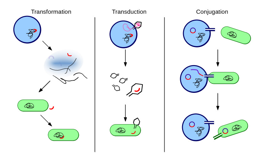
Bacteria, in contrast to eukaryotic cells, contain two types of genes: chromosomal genes that are fixed to the cell, and plasmids, smaller loops of DNA capable of being passed from one cell to another. The sharing of plasmid genes between individual bacteria and between bacterial lineages has contributed vastly to bacterial evolution, allowing specialized traits to 'jump ship' between one lineage or species and the next. The benefits of this generosity from the point of view of both recipient cell and plasmid are generally understood: plasmids receive new hosts and ride out selective sweeps across the population, recipient cells gain new traits (such as antibiotic resistance). Explaining this behavior from the point of view of donor cells is substantially more difficult. Donor cells pay a fitness cost in order to share plasmids, and run the risk of sharing advantageous genes with their competition and rendering their own lineage redundant, while seemingly receiving no benefit in return. Using both compartment based models and agent based simulations we demonstrate that 'secretive' genes which restrict horizontal gene transfer are favored over a wide range of models and parameter values, even when sharing carries no direct cost. 'Generous' chromosomal genes which are more permissive of plasmid transfer are found to have neutral fitness at best, and are generally disfavored by selection. Our findings lead to a peculiar paradox: given the obvious benefits of keeping secrets, why do bacteria share information so freely?

Keywords:

Citation: Alastair D. Jamieson-Lane, Bernd Blasius. The gossip paradox: Why do bacteria share genes?[J]. Mathematical Biosciences and Engineering, 2022, 19(6): 5482-5508. doi: 10.3934/mbe.2022257

Related Papers:

[1]	Erlin Guo, Cuixia Li, Patrick Ling, Fengqin Tang . Convergence rate for integrated self-weighted volatility by using intraday high-frequency data with noise. AIMS Mathematics, 2023, 8(12): 31070-31091. doi: 10.3934/math.20231590
[2]	Wenhui Feng, Xingfa Zhang, Yanshan Chen, Zefang Song . Linear regression estimation using intraday high frequency data. AIMS Mathematics, 2023, 8(6): 13123-13133. doi: 10.3934/math.2023662
[3]	Yue Li, Yunyan Wang . Strong consistency of the nonparametric kernel estimator of the transition density for the second-order diffusion process. AIMS Mathematics, 2024, 9(7): 19015-19030. doi: 10.3934/math.2024925
[4]	Oussama Bouanani, Salim Bouzebda . Limit theorems for local polynomial estimation of regression for functional dependent data. AIMS Mathematics, 2024, 9(9): 23651-23691. doi: 10.3934/math.20241150
[5]	Ahmed Ghezal, Mohamed balegh, Imane Zemmouri . Markov-switching threshold stochastic volatility models with regime changes. AIMS Mathematics, 2024, 9(2): 3895-3910. doi: 10.3934/math.2024192
[6]	Gaosheng Liu, Yang Bai . Statistical inference in functional semiparametric spatial autoregressive model. AIMS Mathematics, 2021, 6(10): 10890-10906. doi: 10.3934/math.2021633
[7]	Junke Kou, Hao Zhang . Wavelet estimations of the derivatives of variance function in heteroscedastic model. AIMS Mathematics, 2023, 8(6): 14340-14361. doi: 10.3934/math.2023734
[8]	Omar Alzeley, Ahmed Ghezal . On an asymmetric multivariate stochastic difference volatility: structure and estimation. AIMS Mathematics, 2024, 9(7): 18528-18552. doi: 10.3934/math.2024902
[9]	Jiajia Zhao, Zuoliang Xu . Calibration of time-dependent volatility for European options under the fractional Vasicek model. AIMS Mathematics, 2022, 7(6): 11053-11069. doi: 10.3934/math.2022617
[10]	Fatimah Alshahrani, Wahiba Bouabsa, Ibrahim M. Almanjahie, Mohammed Kadi Attouch . $k$ NN local linear estimation of the conditional density and mode for functional spatial high dimensional data. AIMS Mathematics, 2023, 8(7): 15844-15875. doi: 10.3934/math.2023809

Abstract

1. Introduction

Many complicated structures' memory and natural features may be realized using fractional calculus (FC), which studies integrals and derivatives of fractional orders ^[1,2]. Many recent FC applications have included analyzing the dynamics of large-scale physical events by converting derivatives and integrals from classical to non-integer order. Many branches of engineering and the physical sciences use it, including electric circuits, mathematical biology, control theory, robotics, viscoelasticity, flow models, relaxation, and signal processing ^[3,4]. Numerous mysterious ideas have been refined via the study of fractional calculus, for example, logistic regression, Malthusian growth, and blood alcohol concentration, all of which have shown that fractional operators outperform integer-order operators ^[5,6].

Derivatives of fractional order such as Riemann-Liouville, Atangana Baleanu, Caputo, Hilfer, Grunwald-Letnikov, Caputo Fabrizio, and Riemann-Liouville are among the numerous that have recently been proposed ^[7,8]. Since all fractional derivatives may be reduced in Caputo's meaning with minor parametric adjustments, the fractional derivative of Caputo is the essential principle of FC to investigate fractional differential equations (FDEs). Caputo's operator, which has numerous applications to model various physical models, possesses a power-law kernel. To address this difficulty, the alternative fractional differential operator ^[9] was developed, which consists of a Mittag-Leffler kernel and an exponentially decaying kernel. Caputo-Fabrizio (CF) and Atangana-Baleanu are operators characterized by their non-singular kernels. These operators have been widely applied in analyzing diverse problem classes, including but not limited to biology, economics, geophysics, and bioengineering ^[10].

Korteweg and de Vries introduced the KdV equation in 1895 to formulate a model for Russell's soliton phenomenon, encompassing water waves of long and small amplitude. Solitons are classified as stable solitary waves, signifying their particle-like nature ^[11]. Various applied disciplines, including plasma physics, fluid dynamics, quantum mechanics, and optics, implement the KdV equations ^[12]. Particle physics has employed the fifth-order KdV equations to analyze many nonlinear phenomena ^[13]. Its function in the propagation of waves is crucial ^[14]. The authors find third-order and fifth-order dispersive terms in the KdV form equation pertinent to the magneto-acoustic wave problem. Furthermore, these dispersive terms manifest themselves in the vicinity of critical angle propagation ^[15]. An electrically conducting fluid, plasma is also dynamic and quasi-neutral. Ions, electrons, and neutral particles comprise it. Due to the electrical conductivity exhibited by plasma, it includes both electric and magnetic regions. The variety of particles and regions supports diverse types of plasma waves. A magnetic lock is a less longitudinal ion dispersion. In the low magnetic field range, the magneto-acoustic wave exhibits characteristics of an ion acoustic wave ^[16,17]. However, at low temperatures, it transforms into an Alfven wave.

Equivalent to the general model for the investigation of magnetic characteristics of acoustic waves with surface tension is the fifth order of KdV. According to a recent investigation ^[18,19], the solutions to the equation above concerning traveling waves persist beyond infinity. The following are two widely recognized types of fifth-order KdV equations ^[20,21]:

$\begin{equation} \begin{split} &D_{{\Omega}}^{p} \eta({\epsilon}, {\Omega})-\frac{\partial ^5\eta({\epsilon}, {\Omega})}{\partial \epsilon^5}+\eta({\epsilon}, {\Omega}) \frac{\partial ^3\eta({\epsilon}, {\Omega})}{\partial \epsilon^3}+\eta({\epsilon}, {\Omega}) \frac{\partial \eta({\epsilon}, {\Omega})}{\partial \epsilon} = 0, \ \ 0 < p \leq 1. \end{split} \end{equation}$

(1.1)

$\begin{equation} \begin{split} &D_{{\Omega}}^{p} \eta({\epsilon}, {\Omega})+\frac{\partial ^5\eta({\epsilon}, {\Omega})}{\partial \epsilon^5}-\eta({\epsilon}, {\Omega}) \frac{\partial ^3\eta({\epsilon}, {\Omega})}{\partial \epsilon^3}+\eta({\epsilon}, {\Omega}) \frac{\partial \eta({\epsilon}, {\Omega})}{\partial \epsilon} = 0, \ \ 0 < p \leq 1. \end{split} \end{equation}$

(1.2)

Here, Eqs (1.1) and (1.2) are called the Kawahara and KdV equation of fifth-order, respectively. The extreme nonlinearity of these mathematical models makes it difficult to find suitable analytical methods. Researchers have developed and implemented several techniques for solving nonlinear and linear equations of KdV in the past ten years. These techniques include the variational iteration method ^[21], the multi-symplectic method ^[22], He's homotopy perturbation method ^[23], and the Exp-function method ^[24].

Omar Abu Arqub established residual power series method (RPSM) in 2013 ^[25]. It is created by merging the residual error function with the Taylor series. According to ^[26], an infinite convergence series solves differential equations (DEs). The development of novel RPSM algorithms has been prompted by several DEs, including KdV Burger's equation, fuzzy DEs, Boussinesq DEs, and numerous others ^[27,28]. The goal of these algorithms is to provide efficient and accurate estimates.

A novel strategy for solving FDEs was established by integrating two effective methods. Some approaches that fall into these categories include those that use the natural transform ^[29], the Laplace transform with RPSM ^[30], and the homotopy perturbation method ^[31]. In this work, we used a novel combination method known as the Abdooh residual power series method (ARPSM) to discover approximation and precise solutions for time-fractional nonlinear partial differential equations (PDEs). This innovative method is significant because it combines the Aboodh transform technique with the RPSM ^[32,33].

The computing effort and complexity needed are significant issues with the previously mentioned approaches. Our suggested Aboodh transform iterative method (ATIM) ^[34] is this work's unique aspect that solves the Kawahara and KdV equations of fractional order. By integrating the Aboodh transform with the new iterative technique, this strategy significantly reduces the computing effort and complexity required. According to ^[35,36], the suggested approach yields a convergent series solution.

The ARPSM and the ATIM are the two most straightforward approaches to solving fractional DEs. These methods fully and immediately explain the symbolic terms used in analytical solutions and offer numerical solutions to PDEs. This paper assesses ATIM and ARPSM's efficacy in solving the fifth-order KdV and Kawahara equations.

The fifth-order KdV and Kawahara equations are solved using ARPSM and ATIM. These methods provide more precise numerical answers when compared with other numerical techniques. Additionally, a comparison analysis is performed on the numerical findings. The suggested approaches' findings are consistent with one another, which is a strong indicator of their efficacy and reliability. For various values of fractional-order derivatives, there is additional graphical importance. Therefore, the methods are accurate, easy to implement, not affected by computational error phases, and quick. This study lays the groundwork for researchers to quickly solve various PDEs.

2. Basics of fractional calculus

Definition 2.1. ^[37] Assume that $\eta({{\epsilon}}, {{\Omega}})$ is an exponential order continuous function. The definition of the Aboodh transform (AT), assuming $\sigma\geq0$ for $\eta({{\epsilon}}, {{\Omega}})$ , is as follows:

$A[\eta({{\epsilon}}, {{\Omega}})] = \Psi({{\epsilon}},\xi) = \frac{1}{\xi}\displaystyle{\int}_{0}^{\infty}\eta({{\epsilon}}, {{\Omega}})e^{-{{\Omega}}\xi}d{{\Omega}},\ \ {r}_{1}\leq\xi\leq{r}_{2}.$

The Aboodh inverse transform (AIT) is given as:

$A^{-1}[\Psi({{\epsilon}},\xi)] = \eta({{\epsilon}}, {{\Omega}}) = \frac{1}{2\pi i}\displaystyle{\int}_{u-i\infty}^{u+i\infty}\Psi({{\epsilon}}, {{\Omega}})\xi e^{{{\Omega}}\xi}d{{\Omega}},$

where ${{\epsilon}} = ({{\epsilon}}_{1}, {{\epsilon}}_{2}, \cdots, {{\epsilon}}_{p})\in \mathbb{R}^{p}$ and $p\in\mathbb{N}$ .

Lemma 2.1. ^[38,39] It is assumed that there exist two exponentially ordered, piecewise continuous functions $\eta_{1}({{\epsilon}}, \Omega)$ and $\eta_{2}({{\epsilon, \Omega}})$ on $[0, \infty]$ . Let $A[\eta_{1}({{\epsilon}}, {{\Omega}})] = \Psi_{1}({{\epsilon}}, {{\Omega}}), A[\eta_{2}({{\epsilon}}, {{\Omega}})] = \Psi_{2}({{\epsilon}}, {{\Omega}})$ , and $\chi_{1}, \chi_{2}$ be arbitrary constants. These characteristics are thus true:

(1) $A[\chi_{1}\eta_{1}({{\epsilon}}, {{\Omega}})+\chi_{2}\eta_{2}({{\epsilon}}, {{\Omega}})] = \chi_{1}\Psi_{1}({{\epsilon}}, \xi)+\chi_{2}\Psi_{2}({{\epsilon}}, {{\Omega}})$ ,

(2) $A^{-1}[\chi_{1}\Psi_{1}({{\epsilon}}, {{\Omega}})+\chi_{2}\Psi_{2}({{\epsilon}}, {{\Omega}})] = \chi_{1}\eta_{1}({{\epsilon}}, \xi)+\chi_{2}\eta_{2}({{\epsilon}}, {{\Omega}})$ ,

(3) $A[J_{{{\Omega}}}^{{p}}\eta({{\epsilon}}, {{\Omega}})] = \frac{\Psi({{\epsilon}}, \xi)}{\xi^{{p}}}$ ,

(4) $A[D_{{{\Omega}}}^{{p}}\eta({{\epsilon}}, {{\Omega}})] = \xi^{{p}}\Psi({{\epsilon}}, \xi)-\sum_{K = 0}^{r-1}\frac{\eta^{K}({{\epsilon}}, 0)}{\xi^{K-{p}+2}}, r-1 < {p}\leq r, \ r\in \mathbb{N}$ .

Definition 2.2. ^[40] In terms of order $p$ , the function $\eta({{\epsilon}}, {{\Omega}})$ has derivative of fractional order as stated by Caputo.

$D_{{{\Omega}}}^{{p}}\eta({{\epsilon}}, {{\Omega}}) = J_{{{\Omega}}}^{m-{p}}\eta^{(m)}({{\epsilon}}, {{\Omega}}), \ m-1 < {p}\leq m,\ r\geq 0,$

where ${{\epsilon}} = ({{\epsilon}}_{1}, {{\epsilon}}_{2}, \cdots, {{\epsilon}}_{p})\in \mathbb{R}^{p}$ and $p, m\in R, J_{{{\Omega}}}^{m-{p}}$ is the integral of the Riemann-Liouville of $\eta({{\epsilon}}, {{\Omega}})$ .

Definition 2.3. ^[41] The representation of power series is composed of the following structure.

$\sum\limits_{r = 0}^{\infty}\hbar_{r}({{\epsilon}})({{\Omega}}-{{\Omega}}_{0})^{r{p}} = 1+\hbar_{1}({{\Omega}}-{{\Omega}}_{0})^{{p}}+\hbar_{2}({{\Omega}}-{{\Omega}}_{0})^{2{p}} +\cdots,$

where ${{\epsilon}} = ({{\epsilon}}_{1}, {{\epsilon}}_{2}, \cdots, {{\epsilon}}_{p})\in \mathbb{R}^{p}$ and $p\in \mathbb{N}$ . This is known as the multiple fractional power series concerning ${{\Omega}}_{0}$ , where ${{\Omega}}$ and $\hbar_{r}({{\epsilon}})'s$ are variable and series coefficients, respectively.

Lemma 2.2. Consider the exponential order function is denoted as $\eta({{\epsilon}}, {{\Omega}})$ . $A[\eta({{\epsilon}}, {{\Omega}})] = \Psi({{\epsilon}}, \xi)$ is the description of the AT in this case. Hence,

$\begin{equation} A[D_{{{\Omega}}}^{r{p}}\eta({{\epsilon}}, {{\Omega}})] = \xi^{r{p}}\Psi({{\epsilon}},\xi)-\sum\limits_{j = 0}^{r-1}\xi^{{p}(r-j)-2}D_{{{\Omega}}}^{j{p}}\eta({{\epsilon}},0), 0 < {p}\leq 1, \end{equation}$

(2.1)

where ${{\epsilon}} = ({{\epsilon}}_{1}, {{\epsilon}}_{2}, \cdots, {{\epsilon}}_{p})\in \mathbb{R}^{p}$ and $p\in \mathbb{N}$ and $D_{{{\Omega}}}^{r{p}} = D_{{{\Omega}}}^{{p}}.D_{{{\Omega}}}^{{p}}.\cdots.D_{{{\Omega}}}^{{p}}(r-times)$

Proof. By using the induction method, we have to prove Eq (2.1). In Eq (2.1), substitute $r = 1$ .

$A[D_{{{\Omega}}}^{{p}}\eta({{\epsilon}}, {{\Omega}})] = \xi^{{p}}\Psi({{\epsilon}},\xi)-\xi^{{p}-2}\eta({{\epsilon}},0)-\xi^{{p}-2}D_{{{\Omega}}}^{{p}}\eta({{\epsilon}},0).$

On the bases of Lemma 2.1, Eq (2.1) for $r = 1$ holds true. Put $r = 2$ in Eq (2.1).

$\begin{equation} A[D_{r}^{2{p}}\eta({{\epsilon}}, {{\Omega}})] = \xi^{2{p}}\Psi({{\epsilon}},\xi)-\xi^{2{p}-2}\eta({{\epsilon}},0)-\xi^{{p}-2}D_{{{\Omega}}}^{{p}}\eta({{\epsilon}},0). \end{equation}$

(2.2)

From left-hand side (LHS) of Eq (2.2), we obtain:

$\begin{equation} LHS = A[D_{{{\Omega}}}^{2{p}}\eta({{\epsilon}}, {{\Omega}})]. \end{equation}$

(2.3)

The expressions for Eq (2.3) are as follows:

$\begin{equation} LHS = A[D_{{{\Omega}}}^{{p}}\eta({{\epsilon}}, {{\Omega}})]. \end{equation}$

(2.4)

Assume

$\begin{equation} z({{\epsilon}}, {{\Omega}}) = D_{{{\Omega}}}^{{p}}\eta({{\epsilon}}, {{\Omega}}). \end{equation}$

(2.5)

This makes Eq (2.4) as

$\begin{equation} LHS = A[D_{{{\Omega}}}^{{p}}z({{\epsilon}}, {{\Omega}})]. \end{equation}$

(2.6)

From the definition of the derivative of Caputo, we make changes in Eq (2.6).

$\begin{equation} LHS = A[J^{1-{p}}z^{'}({{\epsilon}}, {{\Omega}})]. \end{equation}$

(2.7)

By applying the Riemann-Liouville integral Eq (2.7), we obtain:

$\begin{equation} LHS = \frac{A[z^{'}({{\epsilon}}, {{\Omega}})]}{\xi^{1-{p}}}. \end{equation}$

(2.8)

By using the AT feature of differentiability, Eq (2.8) is modified:

$\begin{equation} {{LHS = \xi^{{p}}Z({{\epsilon}},\xi)-\frac{z({{\epsilon}},0)}{\xi^{2-{p}}}.}} \end{equation}$

(2.9)

From Eq (2.5), we derive:

$Z({{\epsilon}},\xi) = \xi^{{p}}\Psi({{\epsilon}},\xi)-\frac{\eta({{\epsilon}},0)}{\xi^{2-{p}}},$

where $A[z({{\epsilon}}, {{\Omega}})] = Z({{\epsilon}}, \xi)$ . Hence, Eq (2.9) becomes

$\begin{equation} LHS = \xi^{2{p}}\Psi({{\epsilon}},\xi)-\frac{\eta({{\epsilon}},0)}{\xi^{2-2{p}}}-\frac{D_{{{\Omega}}}^{{p}}\eta({{\epsilon}},0)}{\xi^{2-{p}}}. \end{equation}$

(2.10)

Let's suppose Eq (2.1) holds true for $r = K$ . Substitute $r = K$ in Eq (2.1):

$\begin{equation} A[D_{{{\Omega}}}^{K{p}}\eta({{\epsilon}}, {{\Omega}})] = \xi^{K{p}}\Psi({{\epsilon}},\xi)-\sum\limits_{j = 0}^{K-1}\xi^{{p}(K-j)-2}D_{{{\Omega}}}^{j{p}}D_{{{\Omega}}}^{j{p}}\eta({{\epsilon}},0),\ 0 < {p}\leq1. \end{equation}$

(2.11)

Substituting $r = K+1$ in Eq (2.1):

$\begin{equation} A[D_{{{\Omega}}}^{(K+1){p}}\eta({{\epsilon}}, {{\Omega}})] = \xi^{(K+1){p}}\Psi({{\epsilon}},\xi)-\sum\limits_{j = 0}^{K}\xi^{{p}((K+1)-j)-2}D_{{{\Omega}}}^{j{p}}\eta({{\epsilon}},0). \end{equation}$

(2.12)

After analyzing Eq (2.12)'s LHS, we deduce

$\begin{equation} LHS = A[D_{{{\Omega}}}^{K{p}}(D_{{{\Omega}}}^{K{p}})]. \end{equation}$

(2.13)

Let

$D_{{{\Omega}}}^{K{p}} = g({{\epsilon}}, {{\Omega}}).$

By Eq (2.13), we drive

$\begin{equation} LHS = A[D_{{{\Omega}}}^{{p}}g({{\epsilon}}, {{\Omega}})]. \end{equation}$

(2.14)

By using the integral of the Riemann-Liouville and derivative of Caputo on Eq (2.14), the subsequent result can be obtained.

$\begin{equation} LHS = \xi^{{p}}A[D_{{{\Omega}}}^{K{p}}\eta({{\epsilon}}, {{\Omega}})]-\frac{g({{\epsilon}},0)}{\xi^{2-{p}}}. \end{equation}$

(2.15)

To get Eq (2.15), use Eq (2.11).

$\begin{equation} LHS = \xi^{r{p}}\Psi({{\epsilon}},\xi)-\sum\limits_{j = 0}^{r-1}\xi^{{p}(r-j)-2}D_{{{\Omega}}}^{j{p}}\eta({{\epsilon}},0). \end{equation}$

(2.16)

In addition, Eq (2.16) produces the subsequent outcome.

$LHS = A[D_{{{\Omega}}}^{r{p}}\eta({{\epsilon}},0)].$

Thus, for $r = K+1$ , Eq (2.1) holds. For all positive integers, Eq (2.1) holds true according to the mathematical induction technique. □

A deeper understanding of the ARPSM and multiple fractional Taylor series (MFTS) are given as follow.

Lemma 2.3. Consider the function $\eta({{\epsilon}}, {{\Omega}})$ is an exponential order. $A[\eta({{\epsilon}}, {{\Omega}})] = \Psi({{\epsilon}}, \xi)$ is the expression that signifies the AT of $\eta({{\epsilon}}, {{\Omega}})$ . AT is represented as follows in MFTS notation:

$\begin{equation} \Psi({{\epsilon}},\xi) = \sum\limits_{r = 0}^{\infty}\frac{\hbar_{r}({{\epsilon}})}{\xi^{r{p}+2}}, \xi > 0, \end{equation}$

(2.17)

where, ${{\epsilon}} = (s_{1}, {{\epsilon}}_{2}, \cdots, {{\epsilon}}_{p})\in\mathbb{R}^{p}, \ p\in \mathbb{N}$ .

Proof. Consider the Taylor's series:

$\begin{equation} \eta({{\epsilon}}, {{\Omega}}) = \hbar_{0}({{\epsilon}})+\hbar_{1}({{\epsilon}})\frac{{{\Omega}}^{{p}}}{\Gamma[{p}+1]}AA+\hbar_{2}({{\epsilon}})\frac{{{\Omega}}^{2{p}}}{\Gamma[2{p}+1]}+\cdots. \end{equation}$

(2.18)

The subsequent equality is produced when the AT is applied to Eq (2.18):

$A\left[\eta({{\epsilon}}, {{\Omega}})\right] = A\left[\hbar_{0}({{\epsilon}})\right]+A\left[\hbar_{1}({{\epsilon}})\frac{{{\Omega}}^{{p}}}{\Gamma[{p}+1]}\right]+A\left[\hbar_{1}({{\epsilon}}) \frac{{{\Omega}}^{2{p}}}{\Gamma[2{p}+1]}\right]+\cdots.$

This is achieved by utilizing the AT's features.

$A\left[\eta({{\epsilon}}, {{\Omega}})\right] = \hbar_{0}({{\epsilon}})\frac{1}{\xi^{2}}+\hbar_{1}({{\epsilon}})\frac{1}{\Gamma[{p}+1]}\frac{1}{\xi^{{p}+2}}+\hbar_{2}({{\epsilon}}) \frac{1}{\Gamma[2{p}+1]}\frac{1}{\xi^{2{p}+2}}\cdots.$

Hence, by Eq (2.17), a new Taylor's series is obtained: □

Lemma 2.4. Let the multiple fractional power series (MFPS) be expressed in terms of Taylor's series new form Eq (2.17), $A[\eta(\epsilon, \Omega)] = \Psi(\epsilon, \xi)$ .

$\begin{equation} \hbar_{0}({{\epsilon}}) = \lim\limits_{\xi\rightarrow \infty}\xi^2\Psi({{\epsilon}},\xi) = \eta({{\epsilon}},0). \end{equation}$

(2.19)

Proof. Let's suppose the Taylor's series:

$\begin{equation} \hbar_{0}({{\epsilon}}) = \xi^2\Psi({{\epsilon}},\xi)-\frac{\hbar_{1}({{\epsilon}})}{\xi^{{p}}}-\frac{\hbar_{2}({{\epsilon}})}{\xi^{2{p}}}-\cdots. \end{equation}$

(2.20)

As denoted by Eq (2.20), the necessary solution can be obtained by employing $lim_{x\rightarrow \infty}$ in Eq (2.19) and performing a short calculation. □

Theorem 2.5. The following is an MFPS representation of the function $A[\eta({{\epsilon}}, {{\Omega}})] = \Psi({{\epsilon}}, \xi)$ :

$\Psi({{\epsilon}},\xi) = \sum\limits_{0}^{\infty}\frac{\hbar_{r}({{\epsilon}})}{\xi^{r{p}+2}}, \ \xi > 0,$

where ${{\epsilon}} = ({{\epsilon}}_{1}, {{\epsilon}}_{2}, \cdots, {{\epsilon}}_{p})\in\mathbb{R}^p$ and $p\in\mathbb{N}$ . Then, we have

$\hbar_{r}({{\epsilon}}) = D_{r}^{r{p}}\eta({{\epsilon}},0),$

where, $D_{{{\Omega}}}^{r{p}} = D_{{{\Omega}}}^{{p}}.D_{{{\Omega}}}^{{p}}.\cdots.D_{{{\Omega}}}^{{p}}(r-times)$ .

Proof. Let's suppose the Taylor's series:

$\begin{equation} \hbar_{1}({{\epsilon}}) = \xi^{{p}+2}\Psi({{\epsilon}},\xi)-\xi^{{p}}\hbar_{0}({{\epsilon}})-\frac{\hbar_{2}({{\epsilon}})}{\xi^{{p}}}-\frac{\hbar_{3}({{\epsilon}})}{\xi^{2{p}}}- \cdots \end{equation}$

(2.21)

$\lim_{\xi\rightarrow \infty}$ , is applied to Eq (2.21), and we get

$\hbar_{1}({{\epsilon}}) = \lim\limits_{\xi\rightarrow \infty}(\xi^{{p}+2}\Psi({{\epsilon}},\xi)-\xi^{{p}}\hbar_{0}({{\epsilon}}))-\lim\limits_{\xi\rightarrow \infty}\frac{\hbar_{2}({{\epsilon}})}{\xi^{{p}}} -\lim\limits_{\xi\rightarrow \infty}\frac{\hbar_{3}({{\epsilon}})}{\xi^{2{p}}}- \cdots.$

The equality that results from taking the limit is as follows:

$\begin{equation} \hbar_{1}({{\epsilon}}) = \lim\limits_{\xi\rightarrow \infty}(\xi^{{p}+2}\Psi({{\epsilon}},\xi)-\xi^{{p}}\hbar_{0}({{\epsilon}})). \end{equation}$

(2.22)

Using Lemma 2.2, we obtain:

$\begin{equation} \hbar_{1}({{\epsilon}}) = \lim\limits_{\xi\rightarrow \infty}(\xi^2A[D_{{{\Omega}}}^{{p}}\eta({{\epsilon}}, {{\Omega}})](\xi)). \end{equation}$

(2.23)

Furthermore, the Eq (2.23) is modified using Lemma 2.3.

$\hbar_{1}({{\epsilon}}) = D_{{{\Omega}}}^{{p}}\eta({{\epsilon}},0).$

Using Taylor's series and applying $limit_{\xi\rightarrow \infty}$ again, we obtain:

$\hbar_{2}({{\epsilon}}) = \xi^{2{p}+2}\Psi({{\epsilon}},\xi)-\xi^{2{p}}\hbar_{0}({{\epsilon}})-\xi^{{p}}\hbar_{1}({{\epsilon}})-\frac{\hbar_{3}({{\epsilon}})}{\xi^{{p}}}- \cdots.$

Lemma 2.3 gives us the result

$\begin{equation} \hbar_2({{\epsilon}}) = \lim\limits_{\xi\rightarrow \infty}\xi^2(\xi^{2{p}}\Psi({{\epsilon}},\xi)-\xi^{2{p}-2}\hbar_{0}({{\epsilon}})-\xi^{{p}-2}\hbar_{1}({{\epsilon}})). \end{equation}$

(2.24)

Equation (2.24) is transformed using Lemmas 2.2 and Eq (2.4).

$\hbar_{2}({{\epsilon}}) = D_{{{\Omega}}}^{2{p}}\eta({{\epsilon}},0).$

Apply the same procedure and Taylor series, and we obtain:

$\hbar_{3}({{\epsilon}}) = \lim\limits_{\xi\rightarrow \infty}\xi^2(A[D_{{{\Omega}}}^{2{p}}\eta({{\epsilon}},{p})](\xi)).$

Finally, we get:

$\hbar_{3}({{\epsilon}}) = D_{{{\Omega}}}^{3{p}}\eta({{\epsilon}},0).$

In general,

$\hbar_{r}({{\epsilon}}) = D_{{{\Omega}}}^{r{p}}\eta({{\epsilon}},0),$

is proved. □ The new Taylor series has the conditions for the convergence given in the subsequent theorem.

Theorem 2.6. The expression for MFTS is given in Lemma 2.3 and can be expressed as: $A [\eta({{\epsilon}}, {{\Omega}})] = \Psi({{\epsilon}}, \xi)$ . When $|\xi^{a}A[D_{{{\Omega}}}^{(K+1){p}}\eta({{\epsilon}}, {{\Omega}})]|\leq T$ , $\forall$ $0 < {p} \leq 1$ , and $0 < \xi \leq s$ , $R_K({{\epsilon}}, \xi)$ is the residual of the new MFTS satisfying:

$|R_{K}({{\epsilon}},\xi)|\leq \frac{T}{\xi^{(K = 1){p}+2}}, \ 0 < \xi\leq s.$

Proof. For $r = 0, 1, 2, \cdots, K + 1$ , and $0 < \xi \leq s$ , we consider to define $A[D_{{{\Omega}}}^{r{p}}\eta({{\epsilon}}, {{\Omega}})](\xi)$ . Utilize the Taylor series to derive the subsequent relation:

$\begin{equation} R_K({{\epsilon}},\xi) = \Psi({{\epsilon}},\xi)-\sum\limits_{r = 0}^K\frac{\hbar_r({{\epsilon}})}{\xi^{r{p}+2}}. \end{equation}$

(2.25)

Apply Theorem 2.5 on Eq (2.25) to obtain:

$\begin{equation} R_K({{\epsilon}},\xi) = \Psi({{\epsilon}},\xi)-\sum\limits_{r = 0}^{K}\frac{D_{{{\Omega}}}^{r{p}}\eta({{\epsilon}},0)}{\xi^{r{p}+2}}. \end{equation}$

(2.26)

$\xi^{(K+1)a+2}$ is to be multiplied with Eq (2.26) to obtain the following form.

$\begin{equation} \xi^{{p}(K+1)+2}R_K({{\epsilon}},\xi) = \xi^{2}(\xi^{{p}(K+1)}\Psi({{\epsilon}},\xi)-\sum\limits_{r = 0}^{K}\xi^{{p}(K+1-r)-2}D_{{{\Omega}}}^{r{p}}\eta({{\epsilon}},0)). \end{equation}$

(2.27)

Equation (2.27) is modified with Lemma 2.2:

$\begin{equation} \xi^{{p}(K+1)+2}R_K({{\epsilon}},\xi) = \xi^{2}A[D_{{{\Omega}}}^{{p}(K+1)}\eta({{\epsilon}}, {{\Omega}})]. \end{equation}$

(2.28)

The absolute of Eq (2.28) gives us

$\begin{equation} |\xi^{{p}(K+1)+2}R_K({{\epsilon}},\xi)| = |\xi^{2}A[D_{{{\Omega}}}^{{p}(K+1)}\eta({{\epsilon}}, {{\Omega}})]|. \end{equation}$

(2.29)

By applying the conditions listed in Eq (2.29), the subsequent result is achieved.

$\begin{equation} \frac{-T}{\xi^{{p}(K+1)+2}}\leq R_K({{\epsilon}},\xi)\leq \frac{T}{\xi^{{p}(K+1)+2}}. \end{equation}$

(2.30)

Equation (2.30) yields the desired outcome.

$|R_K({{\epsilon}},\xi)|\leq \frac{T}{\xi^{{p}(K+1)+2}}.$

Therefore, new conditions for the series to converge are developed. □

3. Methodologies

3.1. ARPSM technique

In this paper, we explain how ARPSM rules formed the basis of our solution.

Step 1: Assume the general PDE:

$\begin{equation} D_{{{\Omega}}}^{q{p}}\eta({{\epsilon}}, {{\Omega}})+\vartheta({{\epsilon}})N(\eta)-\delta({{\epsilon}},\eta) = 0. \\ \end{equation}$

(3.1)

Step 2: Apply the AT on Eq (3.1):

$\begin{equation} A[D_{{{\Omega}}}^{q{p}}\eta({{\epsilon}}, {{\Omega}})+\vartheta({{\epsilon}})N(\eta)-\delta({{\epsilon}},\eta)] = 0. \\ \end{equation}$

(3.2)

Utilizing Lemma 2.1 to modify Eq (3.2),

$\begin{equation} \Psi({{\epsilon}},{s}) = \sum\limits_{j = 0}^{q-1}\frac{D_{{{\Omega}}}^{j}\eta({{\epsilon}},0)}{{s}^{q{p}+2}}-\frac{\vartheta({{\epsilon}})Y({s})}{{s}^{q{p}}}+\frac{F({{\epsilon}},{s})}{{s}^{q{p}}}, \end{equation}$

(3.3)

where $A[\delta({{\epsilon}}, \eta)] = F({{\epsilon}}, {s}), A[N(\eta)] = Y({s})$ .

Step 3: Equation (3.3) takes the following form:

$\Psi({{\epsilon}}, {s}) = \sum\limits_{r = 0}^{\infty}\frac{\hbar_r({{\epsilon}})}{{s}^{r{p}+2}}, \ {s} > 0. \\$

Step 4: Take the steps listed below:

$\hbar_0({{\epsilon}}) = \lim\limits_{{s}\rightarrow \infty}{s}^2 \Psi({{\epsilon}}, {s}) = \eta({{\epsilon}}, 0). \\$

Use Theorem 2.6 to obtain this form.

$\begin{array}{*{20}{c}} {\hbar_{1}({{\epsilon}}) = D_{{{\Omega}}}^{{p}}\eta({{\epsilon}}, 0),}\\ {\hbar_{2}({{\epsilon}}) = D_{{{\Omega}}}^{2{p}}\eta({{\epsilon}}, 0),}\\ {\vdots}\\ {\hbar_{w}({{\epsilon}}) = D_{{{\Omega}}}^{w{p}}\eta({{\epsilon}}, 0).} \end{array}$

Step 5: The $K^{th}$ truncated series $\Psi({{\epsilon}}, {s})$ can be obtained using the following expression:

$\Psi_{K}({{\epsilon}}, {s}) = \sum\limits_{r = 0}^{K}\frac{\hbar_r({{\epsilon}})}{{s}^{r{p}+2}}, \ {s} > 0,$

$\Psi_{K}({{\epsilon}}, {s}) = \frac{\hbar_{0}({{\epsilon}})}{{s}^{2}}+\frac{\hbar_{1}({{\epsilon}})}{{s}^{{p}+2}}+\cdots+\frac{\hbar_{w}({{\epsilon}})}{{s}^{w{p}+2}}+\sum\limits_{r = w+1}^{K} \frac{\hbar_r({{\epsilon}})}{{s}^{r{p}+2}}.$

Step 6: Note that the residual Aboodh function (RAF) (3.3) and the $K^{th}$ -truncated RAF must be considered independently to obtain:

$ARes({{\epsilon}}, {s}) = \Psi({{\epsilon}},{s})-\sum\limits_{j = 0}^{q-1}\frac{D_{{{\Omega}}}^{j}\eta({{\epsilon}},0)}{{s}^{j{p}+2}}+\frac{\vartheta({{\epsilon}})Y({s})}{{s}^{j{p}}}-\frac{F({{\epsilon}},{s})}{{s}^{j{p}}},$

and

$\begin{equation} ARes_{K}({{\epsilon}}, {s}) = \Psi_{K}({{\epsilon}},{s})-\sum\limits_{j = 0}^{q-1}\frac{D_{{{\Omega}}}^{j}\eta({{\epsilon}},0)}{{s}^{j{p}+2}}+\frac{\vartheta({{\epsilon}})Y({s})}{{s}^{j{p}}}-\frac{F({{\epsilon}},{s})}{{s}^{j{p}}}. \end{equation}$

(3.4)

Step 7: Equation (3.4) may be substituted with $\Psi_{K}({{\epsilon}}, {s})$ in place of its expansion form.

$\begin{equation} \begin{split} &ARes_{K}({{\epsilon}}, {s}) = \Big(\frac{\hbar_{0}({{\epsilon}})}{{s}^{2}}+\frac{\hbar_{1}({{\epsilon}})}{{s}^{{p}+2}}+\cdots+\frac{\hbar_{w}({{\epsilon}})}{{s}^{w{p}+2}}+\sum\limits_{r = w+1}^{K} \frac{\hbar_r({{\epsilon}})}{{s}^{r{p}+2}}\Big)\\&-\sum\limits_{j = 0}^{q-1}\frac{D_{{{\Omega}}}^{j}\eta({{\epsilon}},0)}{{s}^{j{p}+2}}+\frac{\vartheta({{\epsilon}})Y({s})}{{s}^{j{p}}} -\frac{F({{\epsilon}},{s})}{{s}^{j{p}}}. \end{split} \end{equation}$

(3.5)

Step 8: Multifly ${s}^{K{p}+2}$ on either side of the equation to get the solution to Eq (3.5).

$\begin{equation} \begin{split} &{s}^{K{p}+2}ARes_{K}({{\epsilon}}, {s}) = {s}^{K{p}+2}\Big(\frac{\hbar_{0}({{\epsilon}})}{{s}^{2}}+\frac{\hbar_{1}({{\epsilon}})}{{s}^{{p}+2}}+\cdots+\frac{\hbar_{w}({{\epsilon}})}{{s}^{w{p}+2}}+\sum\limits_{r = w+1}^{K} \frac{\hbar_r({{\epsilon}})}{{s}^{r{p}+2}}\\&-\sum\limits_{j = 0}^{q-1}\frac{D_{{{\Omega}}}^{j}\eta({{\epsilon}},0)}{{s}^{j{p}+2}}+\frac{\vartheta({{\epsilon}})Y({s})}{{s}^{j{p}}} -\frac{F({{\epsilon}},{s})}{{s}^{j{p}}}\Big). \end{split} \end{equation}$

(3.6)

Step 9: Take $\lim_{{s}\rightarrow \infty}$ of Eq (3.6) to obtain:

$\begin{equation*} \begin{split} &\lim\limits_{{s}\rightarrow \infty}{s}^{K{p}+2}ARes_{K}({{\epsilon}}, {s}) = \lim\limits_{{s}\rightarrow \infty}{s}^{K{p}+2}\Big(\frac{\hbar_{0}({{\epsilon}})}{{s}^{2}}+\frac{\hbar_{1}({{\epsilon}})}{{s}^{{p}+2}}+\cdots+\frac{\hbar_{w}({{\epsilon}})}{{s}^{w{p}+2}}+\sum\limits_{r = w+1}^{K} \frac{\hbar_r({{\epsilon}})}{{s}^{r{p}+2}}\\&-\sum\limits_{j = 0}^{q-1}\frac{D_{{{\Omega}}}^{j}\eta({{\epsilon}},0)}{{s}^{j{p}+2}}+\frac{\vartheta({{\epsilon}})Y({s})}{{s}^{j{p}}} -\frac{F({{\epsilon}},{s})}{{s}^{j{p}}}\Big). \end{split} \end{equation*}$

Step 10: $\hbar_K({{\epsilon}})$ values can be obtained using the equation above.

$\lim\limits_{{s}\rightarrow \infty}({s}^{K{p}+2}ARes_{K}({{\epsilon}}, {s})) = 0,$

where $K = 1+w, 2+w, \cdots.$

Step 11: Values of $\hbar_K({{\epsilon}})$ are then substituted in Eq (3.3).

Step 12: Taking the inverse AT we obtain the final solution $\eta_K({{\epsilon}}, {{\Omega}})$ .

3.2. ATIM Technique

Let's consider the PDE as given below:

$\begin{equation} D_{{{\Omega}}}^{{p}}{{\eta}}({{\epsilon}},{{\Omega}}) = \Phi\Big({{\eta}}({{\epsilon}},{{\Omega}}),D_{{{\epsilon}}}^{\Omega}{{\eta}}({{\epsilon}},{{\Omega}}) ,D_{{{\epsilon}}}^{2\Omega}{{\eta}}({{\epsilon}},{{\Omega}}),D_{{{\epsilon}}}^{3\Omega}{{\eta}}({{\epsilon}},{{\Omega}})\Big),\ 0 < {p},\Omega\leq1. \end{equation}$

(3.7)

The initial condition is

$\begin{equation} {{\eta}}^{(\hbar)}({{\epsilon}},0) = h_{\hbar},\ \hbar = 0,1,2,\cdots,m-1. \end{equation}$

(3.8)

The function to be determined is ${{\eta}}({{\epsilon}}, {{\Omega}})$ , while $\Phi\Big({{\eta}}({{\epsilon}}, {{\Omega}}), D_{{{\epsilon}}}^{\Omega}{{\eta}}({{\epsilon}}, {{\Omega}}), D_{{{\epsilon}}}^{2\Omega}{{\eta}}({{\epsilon}}, {{\Omega}}) D_{{{\epsilon}}}^{3\Omega}{{\eta}}({{\epsilon}}, {{\Omega}})\Big)$ are operators of ${{\eta}}({{\epsilon}}, {{\Omega}}), D_{{{\epsilon}}}^{\Omega}{{\eta}}({{\epsilon}}, {{\Omega}}), D_{{{\epsilon}}}^{2\Omega}{{\eta}}({{\epsilon}}, {{\Omega}})$ and $D_{{{\epsilon}}}^{3\Omega}{{\eta}}({{\epsilon}}, {{\Omega}})$ . The AT is applied on Eq (3.7) to obtain:

$\begin{equation} {A} [{{\eta}}({{\epsilon}},{{\Omega}})] = \frac{1}{{s}^{{p}}}\Big(\sum\limits_{\hbar = 0}^{m-1}\frac{{{\eta}}^{(\hbar)}({{\epsilon}},0)}{{s}^{2-{p}+\hbar}}+{A} \Big[\Phi\Big({{\eta}}({{\epsilon}},{{\Omega}}),D_{{{\epsilon}}}^{\Omega}{{\eta}}({{\epsilon}},{{\Omega}}),D_{{{\epsilon}}}^{2\Omega}{{\eta}}({{\epsilon}},{{\Omega}}),D_{{{\epsilon}}}^{3\Omega}{{\eta}}({{\epsilon}},{{\Omega}})\Big)\Big]\Big). \end{equation}$

(3.9)

The AIT yields the solution to this problem:

$\begin{equation} {{\eta}}({{\epsilon}},{{\Omega}}) = {A}^{-1}\Big[\frac{1}{{s}^{{p}}}\Big(\sum\limits_{\hbar = 0}^{m-1}\frac{{{\eta}}^{(\hbar)}({{\epsilon}},0)}{{s}^{2-{p}+\hbar}}+{A} \Big[\Phi\Big({{\eta}}({{\epsilon}},{{\Omega}}),D_{{{\epsilon}}}^{\Omega}{{\eta}}({{\epsilon}},{{\Omega}}),D_{{{\epsilon}}}^{2\Omega}{{\eta}}({{\epsilon}},{{\Omega}}),D_{{{\epsilon}}}^{3\Omega}{{\eta}}({{\epsilon}},{{\Omega}})\Big)\Big]\Big)\Big]. \end{equation}$

(3.10)

An infinite series denotes the ATIM-derived solution.

$\begin{equation} {{\eta}}({{\epsilon}},{{\Omega}}) = \sum\limits_{i = 0}^{\infty}{{\eta}}_{i}. \end{equation}$

(3.11)

$\Phi\Big({{\eta}}, D_{{{\epsilon}}}^{\Omega}{{\eta}}, D_{{{\epsilon}}}^{2\Omega}{{\eta}}, D_{{{\epsilon}}}^{3\Omega}{{\eta}}\Big)$ can be decomposed as:

$\begin{equation} \begin{split} &\Phi \Big({{\eta}},D_{{{\epsilon}}}^{\Omega}{{\eta}},D_{{{\epsilon}}}^{2\Omega}{{\eta}},D_{{{\epsilon}}}^{3\Omega}{{\eta}}\Big) = \Phi \Big({{\eta}}_{0},D_{{{\epsilon}}}^{\Omega}{{\eta}}_{0},D_{{{\epsilon}}}^{2\Omega}{{\eta}}_{0},D_{{{\epsilon}}}^{3\Omega}{{\eta}}_{0}\Big)\\&+ \sum\limits_{i = 0}^{\infty} \left( \Phi \Big(\sum\limits_{\hbar = 0}^{i}\Big({{\eta}}_{\hbar},D_{{{\epsilon}}}^{\Omega}{{\eta}}_{\hbar},D_{{{\epsilon}}}^{2\Omega}{{\eta}}_{\hbar},D_{{{\epsilon}}}^{3\Omega}{{\eta}}_{\hbar}\Big)\Big) -\Phi \Big(\sum\limits_{\hbar = 1}^{i-1}\Big({{\eta}}_{\hbar},D_{{{\epsilon}}}^{\Omega}{{\eta}}_{\hbar},D_{{{\epsilon}}}^{2\Omega}{{\eta}}_{\hbar},D_{{{\epsilon}}}^{3\Omega}{{\eta}}_{\hbar}\Big)\Big)\right). \end{split} \end{equation}$

(3.12)

The subsequent equation is obtained by substituting the values of Eqs (3.11) and (3.12) for the initial equation (3.10).

$\begin{equation} \begin{split} &\sum\limits_{i = 0}^{\infty}{{\eta}}_i({{\epsilon}},{{\Omega}}) = {A}^{-1}\Big[ \frac{1}{{s}^{{p}}}\Big( \sum\limits_{\hbar = 0}^{m-1}\frac{{{\eta}}^{(\hbar)}({{\epsilon}},0)}{{s}^{2-{p}+\hbar}}+{A}[\Phi ({{\eta}}_{0},D_{{{\epsilon}}}^{\Omega}{{\eta}}_{0},D_{{{\epsilon}}}^{2\Omega}{{\eta}}_{0},D_{{{\epsilon}}}^{3\Omega}{{\eta}}_{0})]\Big)\Big]\\&+{A}^{-1}\Big[ \frac{1}{{s}^{{p}}}\Big({A}\Big[ \sum\limits_{i = 0}^{\infty}\Big(\Phi \sum\limits_{\hbar = 0}^{i}({{\eta}}_{\hbar},D_{{{\epsilon}}}^{\Omega}{{\eta}}_{\hbar},D_{{{\epsilon}}}^{2\Omega}{{\eta}}_{\hbar},D_{{{\epsilon}}}^{3\Omega}{{\eta}}_{\hbar})\Big)\Big]\Big)\Big]\\&-{A}^{-1}\Big[ \frac{1}{{s}^{{p}}}\Big({A}\Big[\Big(\Phi \sum\limits_{\hbar = 1}^{i-1}({{\eta}}_{\hbar},D_{{{\epsilon}}}^{\Omega}{{\eta}}_{\hbar},D_{{{\epsilon}}}^{2\Omega}{{\eta}}_{\hbar},D_{{{\epsilon}}}^{3\Omega}{{\eta}}_{\hbar})\Big)\Big]\Big)\Big] \end{split} \end{equation}$

(3.13)

$\begin{equation} \begin{split} &{{\eta}}_0({{\epsilon}},{{\Omega}}) = {A}^{-1}\Big[ \frac{1}{{s}^{{p}}}\Big( \sum\limits_{\hbar = 0}^{m-1}\frac{{{\eta}}^{(\hbar)}({{\epsilon}},0)}{{s}^{2-{p}+\hbar}}\Big)\Big],\\ &{{\eta}}_1({{\epsilon}},{{\Omega}}) = {A}^{-1}\Big[ \frac{1}{{s}^{{p}}}\Big( {A}[\Phi ({{\eta}}_{0},D_{{{\epsilon}}}^{\Omega}{{\eta}}_{0},D_{{{\epsilon}}}^{2\Omega}{{\eta}}_{0},D_{{{\epsilon}}}^{3\Omega}{{\eta}}_{0})]\Big)\Big],\\ \vdots\\ &{{\eta}}_{m+1}({{\epsilon}},{{\Omega}}) = {A}^{-1}\Big[ \frac{1}{{s}^{{p}}}\Big({A}\Big[ \sum\limits_{i = 0}^{\infty}\Big(\Phi \sum\limits_{\hbar = 0}^{i}({{\eta}}_{\hbar},D_{{{\epsilon}}}^{\Omega}{{\eta}}_{\hbar},D_{{{\epsilon}}}^{2\Omega}{{\eta}}_{\hbar},D_{{{\epsilon}}}^{3\Omega}{{\eta}}_{\hbar})\Big)\Big]\Big)\Big]\\&-{A}^{-1}\Big[ \frac{1}{{s}^{{p}}}\Big({A}\Big[\Big(\Phi \sum\limits_{\hbar = 1}^{i-1}({{\eta}}_{\hbar},D_{{{\epsilon}}}^{\Omega}{{\eta}}_{\hbar},D_{{{\epsilon}}}^{2\Omega}{{\eta}}_{\hbar},D_{{{\epsilon}}}^{3\Omega}{{\eta}}_{\hbar})\Big)\Big]\Big)\Big],\ m = 1,2,\cdots. \end{split} \end{equation}$

(3.14)

For the m-term of Eq (3.7), the analytically approximate solution may be obtained using the following expression:

$\begin{equation} {{\eta}}({{\epsilon}},{{\Omega}}) = \sum\limits_{i = 0}^{m-1}{{\eta}}_{i}. \end{equation}$

(3.15)

4. Application of ARPSM and ATIM

4.1. Example 1 using ARPSM

Consider Kawahara equation of fractional order as follows:

(4.1)

with the initial condition:

$\begin{equation} \begin{split} \eta({\epsilon}, 0) = \frac{105}{169} \text{sech}^4\left(\frac{\epsilon-2}{2 \sqrt{13}}\right), \end{split} \end{equation}$

(4.2)

and exact solution

$\begin{equation*} \begin{split} \eta({\epsilon}, {\Omega}) = \frac{105}{169} \text{sech}^4\left(\frac{-\frac{36 \Omega}{169}+\epsilon-2}{2 \sqrt{13}}\right). \end{split} \end{equation*}$

Equation (4.2) is used, and {AT} is applied to Eq (4.1) to get

$\begin{equation} \begin{split} &\eta({\epsilon}, s)-\frac{\frac{105}{169} \text{sech}^4\left(\frac{\epsilon-2}{2 \sqrt{13}}\right)}{s^2}-\frac{1}{s^p}\Big[\frac{\partial ^5\eta({\epsilon}, s)}{\partial \epsilon^5}\Big]+\frac{1}{s^p}A_{{\Omega}}\Big[A_{{\Omega}}^{-1}\eta({\epsilon}, s)\times \frac{\partial ^3A_{{\Omega}}^{-1}\eta({\epsilon}, s)}{\partial \epsilon^3}\Big]\\&+\frac{1}{s^p}A_{{\Omega}}\Big[A_{{\Omega}}^{-1}\eta({\epsilon}, s)\times \frac{\partial A_{{\Omega}}^{-1}\eta({\epsilon}, s)}{\partial \epsilon}\Big] = 0.\\ \end{split} \end{equation}$

(4.3)

Therefore, the series $k^{th}$ -truncated terms are:

$\begin{equation} \begin{split} \eta({{\epsilon}},s) = \frac{\frac{105}{169} \text{sech}^4\left(\frac{\epsilon-2}{2 \sqrt{13}}\right)}{s^2}+\sum\limits_{r = 1}^{k}\frac{f_{r}({{\epsilon}},s)}{s^{rp+1}}, \ \ r = 1,2,3,4\cdots. \end{split} \end{equation}$

(4.4)

Following is the RAF:

$\begin{equation} \begin{split} &{A}_{{{\Omega}}}Res({{\epsilon}},s) = \eta({\epsilon}, s)-\frac{\frac{105}{169} \text{sech}^4\left(\frac{\epsilon-2}{2 \sqrt{13}}\right)}{s^2}-\frac{1}{s^p}\Big[\frac{\partial ^5\eta({\epsilon}, s)}{\partial \epsilon^5}\Big]+\frac{1}{s^p}A_{{\Omega}}\Big[A_{{\Omega}}^{-1}\eta({\epsilon}, s)\times \frac{\partial ^3A_{{\Omega}}^{-1}\eta({\epsilon}, s)}{\partial \epsilon^3}\Big]\\&+\frac{1}{s^p}A_{{\Omega}}\Big[A_{{\Omega}}^{-1}\eta({\epsilon}, s)\times \frac{\partial A_{{\Omega}}^{-1}\eta({\epsilon}, s)}{\partial \epsilon}\Big] = 0,\\ \end{split} \end{equation}$

(4.5)

and the ${k}^{th}$ -RAFs is:

$\begin{equation} \begin{split} &{A}_{{{\Omega}}}Res_{k}({{\epsilon}},s) = \eta_{k}({\epsilon}, s)-\frac{\frac{105}{169} \text{sech}^4\left(\frac{\epsilon-2}{2 \sqrt{13}}\right)}{s^2}-\frac{1}{s^p}\Big[\frac{\partial ^5\eta_{k}({\epsilon}, s)}{\partial \epsilon^5}\Big]+\frac{1}{s^p}A_{{\Omega}}\Big[A_{{\Omega}}^{-1}\eta_{k}({\epsilon}, s)\times \frac{\partial ^3A_{{\Omega}}^{-1}\eta_{k}({\epsilon}, s)}{\partial \epsilon^3}\Big]\\&+\frac{1}{s^p}A_{{\Omega}}\Big[A_{{\Omega}}^{-1}\eta_{k}({\epsilon}, s)\times \frac{\partial A_{{\Omega}}^{-1}\eta_{k}({\epsilon}, s)}{\partial \epsilon}\Big] = 0.\\ \end{split} \end{equation}$

(4.6)

It takes some calculation to find $f_{r}({{\epsilon}}, s)$ for $r = 1, 2, 3, ...$ . Using these procedures, we replace the $r^{th}$ -truncated series Eq (4.4) for the $r^{th}$ -RAF Eq (4.6), applying $\lim_{s\rightarrow \infty}(s^{r{p}+1})$ and solving ${A}_{{{\Omega}}}Res_{\eta, r}({{\epsilon}}, s)) = 0$ , for $r = 1, 2, 3, \cdots$ . Some terms that we obtain are given below:

$\begin{equation} \begin{split} & f_{1}({{\epsilon}},s) = -\frac{105}{5940688 \sqrt{13}} \Big(17290 \sinh \Big(\frac{\epsilon-2}{2 \sqrt{13}}\Big)-10029 \sinh \Big(\frac{3 (\epsilon-2)}{2 \sqrt{13}}\Big)-2015 \sinh \Big(\frac{5 (\epsilon-2)}{2 \sqrt{13}}\Big)\\&+104 \sinh \Big(\frac{7 (\epsilon-2)}{2 \sqrt{13}}\Big)\Big) \text{sech}^{11}\Big(\frac{\epsilon-2}{2 \sqrt{13}}\Big)\Big),\\ \end{split} \end{equation}$

(4.7)

$\begin{equation} \begin{split} & f_{2}({{\epsilon}},s) = \frac{105}{21718014715904} \Big(50957301372 \cosh \Big(\frac{\epsilon-2}{\sqrt{13}}\Big)+12586770193 \cosh \Big(\frac{2 (\epsilon-2)}{\sqrt{13}}\Big)\\&-12962735946 \cosh \Big(\frac{3 (\epsilon-2)}{\sqrt{13}}\Big)+2020967026 \cosh \Big(\frac{4 (\epsilon-2)}{\sqrt{13}}\Big)+68039374 \cosh \Big(\frac{5 (\epsilon-2)}{\sqrt{13}}\Big)\\&-9200529 \cosh \Big(\frac{6 (\epsilon-2)}{\sqrt{13}}\Big)+43264 \cosh \Big(\frac{7 (\epsilon-2)}{\sqrt{13}}\Big)-54264784626\Big) \text{sech}^{18}\Big(\frac{\epsilon-2}{2 \sqrt{13}}\Big),\\ \end{split} \end{equation}$

(4.8)

and so on.

For $r = 1, 2, 3, \cdots,$ replace $f_{r}({{\epsilon}}, s)$ in Eq (4.4):

$\begin{equation} \begin{split} &\eta({\epsilon},s) = \frac{\frac{105}{169} \text{sech}^4\left(\frac{\epsilon-2}{2 \sqrt{13}}\right)}{s^2}-\Big(\frac{105}{5940688 \sqrt{13}} \Big(17290 \sinh \Big(\frac{\epsilon-2}{2 \sqrt{13}}\Big)-10029 \sinh \Big(\frac{3 (\epsilon-2)}{2 \sqrt{13}}\Big)\\&-2015 \sinh \Big(\frac{5 (\epsilon-2)}{2 \sqrt{13}}\Big)+104 \sinh \Big(\frac{7 (\epsilon-2)}{2 \sqrt{13}}\Big)\Big) \text{sech}^{11}\Big(\frac{\epsilon-2}{2 \sqrt{13}}\Big)\Big)\Big)/\Big(s^{p+1}\Big)\\&+\Big(\frac{105}{21718014715904} \Big(50957301372 \cosh \Big(\frac{\epsilon-2}{\sqrt{13}}\Big)+12586770193 \cosh \Big(\frac{2 (\epsilon-2)}{\sqrt{13}}\Big)\\&-12962735946 \cosh \Big(\frac{3 (\epsilon-2)}{\sqrt{13}}\Big)+2020967026 \cosh \Big(\frac{4 (\epsilon-2)}{\sqrt{13}}\Big)+68039374 \cosh \Big(\frac{5 (\epsilon-2)}{\sqrt{13}}\Big)\\&-9200529 \cosh \Big(\frac{6 (\epsilon-2)}{\sqrt{13}}\Big)+43264 \cosh \Big(\frac{7 (\epsilon-2)}{\sqrt{13}}\Big)-54264784626\Big) \text{sech}^{18}\Big(\frac{\epsilon-2}{2 \sqrt{13}}\Big)\Big)/\Big(s^{2p+1}\Big)+\cdots.\\ \end{split} \end{equation}$

(4.9)

Apply AIT to obtain:

$\begin{equation} \begin{split} &\eta({\epsilon},{\Omega}) = \frac{105}{169} \text{sech}^4\left(\frac{\epsilon-2}{2 \sqrt{13}}\right)-\Omega^p\Big(\frac{105}{5940688 \sqrt{13}} \Big(17290 \sinh \Big(\frac{\epsilon-2}{2 \sqrt{13}}\Big)-10029 \sinh \Big(\frac{3 (\epsilon-2)}{2 \sqrt{13}}\Big)\\&-2015 \sinh \Big(\frac{5 (\epsilon-2)}{2 \sqrt{13}}\Big)+104 \sinh \Big(\frac{7 (\epsilon-2)}{2 \sqrt{13}}\Big)\Big) \text{sech}^{11}\Big(\frac{\epsilon-2}{2 \sqrt{13}}\Big)\Big)\Big)/\Big(\Gamma(p+1)\Big)\\&+\Omega^{2p}\Big(\frac{105}{21718014715904} \Big(50957301372 \cosh \Big(\frac{\epsilon-2}{\sqrt{13}}\Big)+12586770193 \cosh \Big(\frac{2 (\epsilon-2)}{\sqrt{13}}\Big)\\&-12962735946 \cosh \Big(\frac{3 (\epsilon-2)}{\sqrt{13}}\Big)+2020967026 \cosh \Big(\frac{4 (\epsilon-2)}{\sqrt{13}}\Big)+68039374 \cosh \Big(\frac{5 (\epsilon-2)}{\sqrt{13}}\Big)\\&-\!9200529 \cosh \Big(\frac{6 (\epsilon-2)}{\sqrt{13}}\Big)\!+\!43264 \cosh \Big(\frac{7 (\epsilon-2)}{\sqrt{13}}\Big)\!-\!54264784626\Big) \text{sech}^{18}\Big(\frac{\epsilon-2}{2 \sqrt{13}}\Big)\Big)/\Big(\Gamma(2p+1)\Big)\!+\!\cdots.\\ \end{split} \end{equation}$

(4.10)

presents the ARPSM solution comparison for different values of the parameter $p$ for $\Omega = 0.1$ , illustrating how the choice of $p$ impacts the accuracy and behavior of the solutions. shows a comparison between the approximate solution obtained using ARPSM (a) and the exact solution (b) for Example 1, confirming the high accuracy of the ARPSM approach. visualizes the impact of varying fractional orders on the ARPSM solution for different $p$ values $(p = 0.32, 0.52, 0.72)$ , showcasing how changes in the fractional order influence the solution structure. extends the comparison in two dimensions, offering a 2D view of the fractional order solutions using ARPSM for the same values of $p$ , further confirming the method's ability to capture the dynamics of fractional systems.

Table 1. ARPSM solution comparison for the values of p of Example 1 for

$\Omega = 0.1$ .

$\epsilon$	$ARPSM_{p=0.52}$	$ARPSM_{p=0.72}$	$ARPSM_{p=1.00}$	$Exact$	$Error_{p=1.00}$
1.0	0.597480	0.597823	0.597918	0.597923	4.746940 $\times 10^{-6}$
1.1	0.601882	0.602193	0.602280	0.602284	4.296239 $\times 10^{-6}$
1.2	0.605857	0.606136	0.606214	0.606217	3.837431 $\times 10^{-6}$
1.3	0.609395	0.609642	0.609710	0.609713	3.371748 $\times 10^{-6}$
1.4	0.612487	0.612700	0.612759	0.612762	2.900316 $\times 10^{-6}$
1.5	0.615125	0.615304	0.615354	0.615356	2.424166 $\times 10^{-6}$
1.6	0.617301	0.617446	0.617486	0.617488	1.944232 $\times 10^{-6}$
1.7	0.619010	0.619121	0.619151	0.619152	1.461368 $\times 10^{-6}$
1.8	0.620248	0.620324	0.620344	0.620345	9.763596 $\times 10^{-7}$
1.9	0.621010	0.621051	0.621061	0.621062	4.899361 $\times 10^{-7}$
2.0	0.621296	0.621301	0.621302	0.621302	2.792130 $\times 10^{-8}$

| Show Table

DownLoad: CSV

Figure 1. (a) ARPSM approximate solution, (b) exact solution.

DownLoad: Full-Size Img PowerPoint

Figure 2. Fractional order comparison using ARPSM for

$p = 0.32, 0.52, 0.72$ .

DownLoad: Full-Size Img PowerPoint

Figure 3. Fractional order 2D comparison using ARPSM for

$p = 0.32, 0.52, 0.72$ .

DownLoad: Full-Size Img PowerPoint

4.2. Example 1 using ATIM

Consider the Kawahara equation of fractional order:

$\begin{equation} \begin{split} &D_{{\Omega}}^{p} \eta({\epsilon}, {\Omega}) = \frac{\partial ^5\eta({\epsilon}, {\Omega})}{\partial \epsilon^5}-\eta({\epsilon}, {\Omega}) \frac{\partial ^3\eta({\epsilon}, {\Omega})}{\partial \epsilon^3}-\eta({\epsilon}, {\Omega}) \frac{\partial \eta({\epsilon}, {\Omega})}{\partial \epsilon}, \ \ \text { where }\ \ 0 < p \leq 1, \end{split} \end{equation}$

(4.11)

with the initial condition:

$\begin{equation} \begin{split} \eta({\epsilon}, 0) = \frac{105}{169} \text{sech}^4\left(\frac{\epsilon-2}{2 \sqrt{13}}\right), \end{split} \end{equation}$

(4.12)

and exact solution

$\begin{equation*} \begin{split} \eta({\epsilon}, {\Omega}) = \frac{105}{169} \text{sech}^4\left(\frac{-\frac{36 \Omega}{169}+\epsilon-2}{2 \sqrt{13}}\right). \end{split} \end{equation*}$

Apply AT on both sides of Eq (4.11) to obtain:

$\begin{equation} {A} [D_{{\Omega}}^{p} \eta({\epsilon}, {\Omega})] = \frac{1}{{s}^{{p}}}\Big(\sum\limits_{k = 0}^{m-1}\frac{\eta^{(k)}({{\epsilon}},0)}{{s}^{2-{p}+k}}+{A} \Big[\frac{\partial ^5\eta({\epsilon}, {\Omega})}{\partial \epsilon^5}-\eta({\epsilon}, {\Omega}) \frac{\partial ^3\eta({\epsilon}, {\Omega})}{\partial \epsilon^3}-\eta({\epsilon}, {\Omega}) \frac{\partial \eta({\epsilon}, {\Omega})}{\partial \epsilon}\Big]\Big). \end{equation}$

(4.13)

Apply AIT on Eq (4.13) to obtain:

$\begin{equation} \eta({\epsilon}, {\Omega}) = {A}^{-1}\Big[\frac{1}{{s}^{{p}}}\Big(\sum\limits_{k = 0}^{m-1}\frac{\eta^{(k)}({{\epsilon}},0)}{{s}^{2-{p}+k}}+{A} \Big[\frac{\partial ^5\eta({\epsilon}, {\Omega})}{\partial \epsilon^5}-\eta({\epsilon}, {\Omega}) \frac{\partial ^3\eta({\epsilon}, {\Omega})}{\partial \epsilon^3}-\eta({\epsilon}, {\Omega}) \frac{\partial \eta({\epsilon}, {\Omega})}{\partial \epsilon}\Big]\Big)\Big]. \end{equation}$

(4.14)

Utilize AT iteratively to get:

$\begin{equation*} \begin{split} \eta_0({\epsilon}, {\Omega}) = &{A}^{-1}\Big[\frac{1}{{s}^{{p}}}\Big(\sum\limits_{k = 0}^{m-1}\frac{\eta^{(k)}({{\epsilon}},0)}{{s}^{2-{p}+k}}\Big)\Big]\\& = {A}^{-1}\Big[\frac{\eta({{\epsilon}},0)}{{s}^2}\Big]\\& = \frac{105}{169} \text{sech}^4\left(\frac{\epsilon-2}{2 \sqrt{13}}\right). \end{split} \end{equation*}$

Applying the Riemann-Liouville integral on Eq (4.11),

$\begin{equation} \begin{split} &\eta({\epsilon}, {\Omega}) = \frac{105}{169} \text{sech}^4\left(\frac{\epsilon-2}{2 \sqrt{13}}\right)-{A}\Big[\frac{\partial ^5\eta({\epsilon}, {\Omega})}{\partial \epsilon^5}-\eta({\epsilon}, {\Omega}) \frac{\partial ^3\eta({\epsilon}, {\Omega})}{\partial \epsilon^3}-\eta({\epsilon}, {\Omega}) \frac{\partial \eta({\epsilon}, {\Omega})}{\partial \epsilon}\Big].\\ \end{split} \end{equation}$

(4.15)

Using the ATIM technique, we provide the following terms:

$\begin{equation} \begin{split} &\eta_{0}({\epsilon},{\Omega}) = \frac{105}{169} \text{sech}^4\left(\frac{\epsilon-2}{2 \sqrt{13}}\right),\\ &\eta_{1}({\epsilon},{\Omega}) = \frac{105}{2970344 \sqrt{13} \Gamma (p+1)} \Omega ^p \Big(11940 \cosh \Big(\frac{\epsilon -2}{\sqrt{13}}\Big)+1911 \cosh \Big(\frac{2 (\epsilon -2)}{\sqrt{13}}\Big)-104 \cosh \Big(\frac{3 (\epsilon -2)}{\sqrt{13}}\Big)\\&-2675\Big) \tanh \Big(\frac{\epsilon -2}{2 \sqrt{13}}\Big) \text{sech}^{10}\Big(\frac{\epsilon -2}{2 \sqrt{13}}\Big),\\ &\eta_{2}({\epsilon},{\Omega}) = \frac{105 \Omega ^{2 p} \text{sech}^{18}\Big(\frac{\epsilon -2}{2 \sqrt{13}}\Big)}{620288218300934144} \Big(\Big(35 \sqrt{\frac{13}{\pi }} 4^p \Omega ^p \Gamma \Big(p+\frac{1}{2}\Big) \Big(13 \Big(9385221 \sinh \Big(\frac{1}{2} \sqrt{13} (\epsilon -2)\Big)\\&+120132725 \sinh \Big(\frac{11 (\epsilon -2)}{2 \sqrt{13}}\Big)-910000 \sinh \Big(\frac{15 (\epsilon -2)}{2 \sqrt{13}}\Big)+14144 \sinh \Big(\frac{17 (\epsilon -2)}{2 \sqrt{13}}\Big)\Big)\\&+581521261600 \sinh \Big(\frac{\epsilon -2}{2 \sqrt{13}}\Big)-374464577051 \sinh \Big(\frac{3 (\epsilon -2)}{2 \sqrt{13}}\Big)+130226023125 \sinh \Big(\frac{5 (\epsilon -2)}{2 \sqrt{13}}\Big)\\ -&12004154204 \sinh \Big(\frac{7 (\epsilon -2)}{2 \sqrt{13}}\Big)-7059672300 \sinh \Big(\frac{9 (\epsilon -2)}{2 \sqrt{13}}\Big)\Big) \text{sech}^7\Big(\frac{\epsilon -2}{2 \sqrt{13}}\Big)\Big)/\Big(p^2 \Gamma (p) \Gamma (3 p)\Big)\\+&\frac{28561}{\Gamma (2 p+1)} \Big(50957301372 \cosh \Big(\frac{\epsilon -2}{\sqrt{13}}\Big)+12586770193 \cosh \Big(\frac{2 (\epsilon -2)}{\sqrt{13}}\Big)\\-&12962735946 \cosh \Big(\frac{3 (\epsilon -2)}{\sqrt{13}}\Big)+13 \Big(155459002 \cosh \Big(\frac{4 (\epsilon -2)}{\sqrt{13}}\Big)+5233798 \cosh \Big(\frac{5 (\epsilon -2)}{\sqrt{13}}\Big)\\-&707733 \cosh \Big(\frac{6 (\epsilon -2)}{\sqrt{13}}\Big)+3328 \cosh \Big(\frac{7 (\epsilon -2)}{\sqrt{13}}\Big)-4174214202\Big)\Big)\Big). \end{split} \end{equation}$

(4.16)

The final solution that is obtained via ATIM is given as:

$\begin{equation} \begin{split} \eta({\epsilon},{\Omega}) = \eta_{0}({\epsilon},{\Omega})+\eta_{1}({\epsilon},{\Omega})+\eta_{2}({\epsilon},{\Omega})+\cdots. \end{split} \end{equation}$

(4.17)

$\begin{equation} \begin{split} &\eta({\epsilon},{\Omega}) = \frac{105}{169} \text{sech}^4\left(\frac{\epsilon-2}{2 \sqrt{13}}\right)+\frac{105}{2970344 \sqrt{13} \Gamma (p+1)} \Omega ^p \Big(11940 \cosh \Big(\frac{\epsilon -2}{\sqrt{13}}\Big)\\&+1911 \cosh \Big(\frac{2 (\epsilon -2)}{\sqrt{13}}\Big)-104 \cosh \Big(\frac{3 (\epsilon -2)}{\sqrt{13}}\Big)-2675\Big) \tanh \Big(\frac{\epsilon -2}{2 \sqrt{13}}\Big) \text{sech}^{10}\Big(\frac{\epsilon -2}{2 \sqrt{13}}\Big)\\&+\frac{105 \Omega ^{2 p} \text{sech}^{18}\Big(\frac{\epsilon -2}{2 \sqrt{13}}\Big)}{620288218300934144} \Big(\Big(35 \sqrt{\frac{13}{\pi }} 4^p \Omega ^p \Gamma \Big(p+\frac{1}{2}\Big) \Big(13 \Big(9385221 \sinh \Big(\frac{1}{2} \sqrt{13} (\epsilon -2)\Big)\\&+120132725 \sinh \Big(\frac{11 (\epsilon -2)}{2 \sqrt{13}}\Big)-910000 \sinh \Big(\frac{15 (\epsilon -2)}{2 \sqrt{13}}\Big)+14144 \sinh \Big(\frac{17 (\epsilon -2)}{2 \sqrt{13}}\Big)\Big)\\&+581521261600 \sinh \Big(\frac{\epsilon -2}{2 \sqrt{13}}\Big)-374464577051 \sinh \Big(\frac{3 (\epsilon -2)}{2 \sqrt{13}}\Big)+130226023125 \sinh \Big(\frac{5 (\epsilon -2)}{2 \sqrt{13}}\Big)\\&-12004154204 \sinh \Big(\frac{7 (\epsilon -2)}{2 \sqrt{13}}\Big)-7059672300 \sinh \Big(\frac{9 (\epsilon -2)}{2 \sqrt{13}}\Big)\Big) \text{sech}^7\Big(\frac{\epsilon -2}{2 \sqrt{13}}\Big)\Big)/\Big(p^2 \Gamma (p) \Gamma (3 p)\Big)\\ &+\frac{28561}{\Gamma (2 p+1)} \Big(50957301372 \cosh \Big(\frac{\epsilon -2}{\sqrt{13}}\Big)+12586770193 \cosh \Big(\frac{2 (\epsilon -2)}{\sqrt{13}}\Big)\\&-12962735946 \cosh \Big(\frac{3 (\epsilon -2)}{\sqrt{13}}\Big)+13 \Big(155459002 \cosh \Big(\frac{4 (\epsilon -2)}{\sqrt{13}}\Big)+5233798 \cosh \Big(\frac{5 (\epsilon -2)}{\sqrt{13}}\Big)\\&-707733 \cosh \Big(\frac{6 (\epsilon -2)}{\sqrt{13}}\Big)+3328 \cosh \Big(\frac{7 (\epsilon -2)}{\sqrt{13}}\Big)-4174214202\Big)\Big)\Big)+\cdots.\\ \end{split} \end{equation}$

(4.18)

compares ATIM solutions for the same set of parameters, with similar trends observed as in ARPSM, demonstrating the robustness of both methods. juxtaposes the ATIM approximate solution (a) with the exact solution (b), verifying the precision of the ATIM method. compares the fractional order solutions using ATIM for $(p = 0.32, 0.52, 0.72)$ , and presents a 2D version of this comparison, highlighting the impact of the fractional order on the solution dynamics. compares the absolute error for ARPSM and ATIM at $\Omega = 0.1$ , demonstrating that both methods achieve highly accurate solutions with minimal error.

Table 2. ATIM solution comparison for the values of p of Example 1 for

$\Omega = 0.1$ .

$\epsilon$	$ATIM_{p=0.52}$	$ATIM_{p=0.72}$	$ATIM_{p=1.00}$	$Exact$	$Error_{p=1.00}$
1.0	0.597546	0.597850	0.597917	0.597923	6.195481 $\times 10^{-6}$
1.1	0.601942	0.602218	0.602278	0.602284	5.609848 $\times 10^{-6}$
1.2	0.605911	0.606158	0.606212	0.606217	5.012997 $\times 10^{-6}$
1.3	0.609443	0.609661	0.609709	0.609713	4.406507 $\times 10^{-6}$
1.4	0.612528	0.612717	0.612758	0.612762	3.791852 $\times 10^{-6}$
1.5	0.615160	0.615318	0.615353	0.615356	3.170410 $\times 10^{-6}$
1.6	0.617329	0.617458	0.617485	0.617488	2.543461 $\times 10^{-6}$
1.7	0.619032	0.619130	0.619150	0.619152	1.912204 $\times 10^{-6}$
1.8	0.620263	0.620329	0.620343	0.620345	1.277767 $\times 10^{-6}$
1.9	0.621019	0.621054	0.621061	0.621062	6.412226 $\times 10^{-7}$
2.0	0.621298	0.621302	0.621302	0.621302	3.606186 $\times 10^{-8}$

| Show Table

DownLoad: CSV

Figure 4. (a) ATIM approximate solution, (b) exact solution.

DownLoad: Full-Size Img PowerPoint

Figure 5. Fractional order comparison using ATIM for

$p = 0.32, 0.52, 0.72$ .

DownLoad: Full-Size Img PowerPoint

Figure 6. Fractional order 2D comparison using ATIM for

$p = 0.32, 0.52, 0.72$ .

DownLoad: Full-Size Img PowerPoint

Table 3. The comparison of absolute error of Example 1 for

$\Omega = 0.1$ .

$\epsilon$	$ARPSM_{p=1}$	$ATIM_{p=1}$	$Exact$	$Error_{ARPSM}$	$Error_{ATIM}$
1.0	0.597918	0.597917	0.597923	4.746940 $\times 10^{-6}$	6.195481 $\times 10^{-6}$
1.1	0.602280	0.602278	0.602284	4.296239 $\times 10^{-6}$	5.609848 $\times 10^{-6}$
1.2	0.606214	0.606212	0.606217	3.837431 $\times 10^{-6}$	5.012997 $\times 10^{-6}$
1.3	0.609710	0.609709	0.609713	3.371748 $\times 10^{-6}$	4.406507 $\times 10^{-6}$
1.4	0.612759	0.612758	0.612762	2.900316 $\times 10^{-6}$	3.791852 $\times 10^{-6}$
1.5	0.615354	0.615353	0.615356	2.424166 $\times 10^{-6}$	3.170410 $\times 10^{-6}$
1.6	0.617486	0.617485	0.617488	1.944232 $\times 10^{-6}$	2.543461 $\times 10^{-6}$
1.7	0.619151	0.619150	0.619152	1.461368 $\times 10^{-6}$	1.912204 $\times 10^{-6}$
1.8	0.620344	0.620343	0.620345	9.763596 $\times 10^{-7}$	1.277767 $\times 10^{-6}$
1.9	0.621061	0.621061	0.621062	4.899361 $\times 10^{-7}$	6.412226 $\times 10^{-7}$
2.0	0.621302	0.621302	0.621302	2.792130 $\times 10^{-8}$	3.606186 $\times 10^{-8}$

| Show Table

DownLoad: CSV

4.3. Example 2 using ARPSM

Examine the famous fifth-order KdV equations as follows:

(4.19)

with the initial condition:

$\begin{equation} \begin{split} \eta({\epsilon},0) = e^{\epsilon}, \end{split} \end{equation}$

(4.20)

and exact solution

$\begin{equation*} \begin{split} \eta({\epsilon},{\Omega}) = e^{\epsilon-\Omega}. \end{split} \end{equation*}$

After applying AT to Eq (4.19), Eq (4.20) is used to obtain:

$\begin{equation} \begin{split} &\eta({\epsilon}, s)-\frac{e^{\epsilon}}{s^2}+\frac{1}{s^p}\Big[\frac{\partial ^5\eta({\epsilon}, s)}{\partial \epsilon^5}\Big]-\frac{1}{s^p}A_{{\Omega}}\Big[A_{{\Omega}}^{-1}\eta({\epsilon}, s)\times \frac{\partial ^3A_{{\Omega}}^{-1}\eta({\epsilon}, s)}{\partial \epsilon^3}\Big]\\&+\frac{1}{s^p}A_{{\Omega}}\Big[A_{{\Omega}}^{-1}\eta({\epsilon}, s)\times \frac{\partial A_{{\Omega}}^{-1}\eta({\epsilon}, s)}{\partial \epsilon}\Big] = 0.\\ \end{split} \end{equation}$

(4.21)

Therefore, the $k^{th}$ -truncated term series is:

$\begin{equation} \begin{split} \eta({{\epsilon}},s) = \frac{e^{\epsilon}}{s^2}+\sum\limits_{r = 1}^{k}\frac{f_{r}({{\epsilon}},s)}{s^{rp+1}}, \ \ r = 1,2,3,4\cdots. \end{split} \end{equation}$

(4.22)

Following is the RAF:

$\begin{equation} \begin{split} &{A}_{{{\Omega}}}Res({{\epsilon}},s) = \eta({\epsilon}, s)-\frac{e^{\epsilon}}{s^2}+\frac{1}{s^p}\Big[\frac{\partial ^5\eta({\epsilon}, s)}{\partial \epsilon^5}\Big]-\frac{1}{s^p}A_{{\Omega}}\Big[A_{{\Omega}}^{-1}\eta({\epsilon}, s)\times \frac{\partial ^3A_{{\Omega}}^{-1}\eta({\epsilon}, s)}{\partial \epsilon^3}\Big]\\&+\frac{1}{s^p}A_{{\Omega}}\Big[A_{{\Omega}}^{-1}\eta({\epsilon}, s)\times \frac{\partial A_{{\Omega}}^{-1}\eta({\epsilon}, s)}{\partial \epsilon}\Big] = 0,\\ \end{split} \end{equation}$

(4.23)

and the ${k}^{th}$ -RAFs is:

$\begin{equation} \begin{split} &{A}_{{{\Omega}}}Res_{k}({{\epsilon}},s) = \eta_{k}({\epsilon}, s)-\frac{e^{\epsilon}}{s^2}+\frac{1}{s^p}\Big[\frac{\partial ^5\eta_{k}({\epsilon}, s)}{\partial \epsilon^5}\Big]-\frac{1}{s^p}A_{{\Omega}}\Big[A_{{\Omega}}^{-1}\eta_{k}({\epsilon}, s)\times \frac{\partial ^3A_{{\Omega}}^{-1}\eta_{k}({\epsilon}, s)}{\partial \epsilon^3}\Big]\\&+\frac{1}{s^p}A_{{\Omega}}\Big[A_{{\Omega}}^{-1}\eta_{k}({\epsilon}, s)\times \frac{\partial A_{{\Omega}}^{-1}\eta_{k}({\epsilon}, s)}{\partial \epsilon}\Big] = 0.\\ \end{split} \end{equation}$

(4.24)

It takes some calculation to find $f_{r}({{\epsilon}}, s)$ for $r = 1, 2, 3, ...$ . Using these procedures, we replace the $r^{th}$ -truncated series Eq (4.22) for the $r^{th}$ -RAF Eq (4.24), applying $\lim_{s\rightarrow \infty}(s^{r{p}+1})$ and solving ${A}_{{{\Omega}}}Res_{\eta, r}({{\epsilon}}, s)) = 0$ , for $r = 1, 2, 3, \cdots$ .

$\begin{equation} \begin{split} & f_{1}({{\epsilon}},s) = -e^{\epsilon},\\ \end{split} \end{equation}$

(4.25)

$\begin{equation} \begin{split} &f_{2}({\epsilon},s) = e^{\epsilon},\\ \end{split} \end{equation}$

(4.26)

$\begin{equation} \begin{split} &f_{2}({\epsilon},s) = -e^{\epsilon},\\ \end{split} \end{equation}$

(4.27)

and so on.

For $r = 1, 2, 3, \cdots,$ replace $f_{r}({{\epsilon}}, s)$ in Eq (4.22):

$\begin{equation} \begin{split} &\eta({\epsilon},s) = \frac{e^\epsilon}{s}-\frac{e^\epsilon}{s^{p+1}}+\frac{e^\epsilon}{s^{2 p+1}}-\frac{e^\epsilon}{s^{3 p+1}}+\cdots.\\ \end{split} \end{equation}$

(4.28)

Apply AIT to obtain:

$\begin{equation} \begin{split} &\eta({\epsilon},{\Omega}) = e^\epsilon-\frac{e^\epsilon \Omega^p}{\Gamma (p+1)}+\frac{e^\epsilon \Omega^{2 p}}{\Gamma (2 p+1)}-\frac{e^\epsilon \Omega^{4 p}}{\Gamma (3 p+1)}+\cdots.\\ \end{split} \end{equation}$

(4.29)

explores the fractional order comparison using ARPSM for an extended range of $p$ values $(p = 0.33, 0.55, 0.77, 1.00)$ , providing a more comprehensive analysis of how different orders affect the solution. Figure 8 offers 2D and 3D graphs for ARPSM solutions, further highlighting the changes in solution behavior as the fractional order varies.

Figure 7. Fractional order comparison using ARPSM for

$p = 0.33, 0.55, 0.77, 1.00$ .

DownLoad: Full-Size Img PowerPoint

Figure 8. 2D and 3D graphs for comparing ARPSM solution for

$p = 0.33, 0.55, 0.77, 1.00$ .

DownLoad: Full-Size Img PowerPoint

4.4. Example 2 using ATIM

Examine the famous fifth-order KdV equations as follows:

$\begin{equation} \begin{split} &D_{{\Omega}}^{p} \eta({\epsilon}, {\Omega}) = -\frac{\partial ^5\eta({\epsilon}, {\Omega})}{\partial \epsilon^5}+\eta({\epsilon}, {\Omega}) \frac{\partial ^3\eta({\epsilon}, {\Omega})}{\partial \epsilon^3}-\eta({\epsilon}, {\Omega}) \frac{\partial \eta({\epsilon}, {\Omega})}{\partial \epsilon}, \ \ \text { where }\ \ 0 < p \leq 1, \end{split} \end{equation}$

(4.30)

with the initial condition:

$\begin{equation} \begin{split} \eta({\epsilon},0) = e^{\epsilon}, \end{split} \end{equation}$

(4.31)

and exact solution

$\begin{equation*} \begin{split} \eta({\epsilon},{\Omega}) = e^{\epsilon-\Omega}. \end{split} \end{equation*}$

Apply AT on either side of Eq (4.30) to obtain:

$\begin{equation} \begin{split} {A} [D_{{\Omega}}^{p} \eta({\epsilon},{\Omega})] = \frac{1}{{s}^{{p}}}\Big(\sum\limits_{k = 0}^{m-1}\frac{\eta^{(k)}({{\epsilon}},0)}{{s}^{2-{p}+k}}+{A} \Big[-\frac{\partial ^5\eta({\epsilon}, {\Omega})}{\partial \epsilon^5}+\eta({\epsilon}, {\Omega}) \frac{\partial ^3\eta({\epsilon}, {\Omega})}{\partial \epsilon^3}-\eta({\epsilon}, {\Omega}) \frac{\partial \eta({\epsilon}, {\Omega})}{\partial \epsilon}\Big]\Big). \end{split} \end{equation}$

(4.32)

Apply AIT on either side of Eq (4.32) to obtain:

$\begin{equation} \begin{split} \eta({\epsilon}, {\Omega}) = {A}^{-1}\Big[\frac{1}{{s}^{{p}}}\Big(\sum\limits_{k = 0}^{m-1}\frac{\eta^{(k)}({{\epsilon}},0)}{{s}^{2-{p}+k}}+{A} \Big[-\frac{\partial ^5\eta({\epsilon}, {\Omega})}{\partial \epsilon^5}+\eta({\epsilon}, {\Omega}) \frac{\partial ^3\eta({\epsilon}, {\Omega})}{\partial \epsilon^3}-\eta({\epsilon}, {\Omega}) \frac{\partial \eta({\epsilon}, {\Omega})}{\partial \epsilon}\Big]\Big)\Big]. \end{split} \end{equation}$

(4.33)

Iteratively apply the AT to obtain:

Applying Riemann-Liouville integral on Eq (4.19),

$\begin{equation} \begin{split} &\eta({\epsilon},{\Omega}) = e^{\epsilon}- {A}\Big[-\frac{\partial ^5\eta({\epsilon}, {\Omega})}{\partial \epsilon^5}+\eta({\epsilon}, {\Omega}) \frac{\partial ^3\eta({\epsilon}, {\Omega})}{\partial \epsilon^3}-\eta({\epsilon}, {\Omega}) \frac{\partial \eta({\epsilon}, {\Omega})}{\partial \epsilon}\Big].\\ \end{split} \end{equation}$

(4.34)

The use of the ATIM technique provides the following terms:

$\begin{equation} \begin{split} &\eta_{0}({\epsilon},{\Omega}) = e^{\epsilon},\\ &\eta_{1}({\epsilon},{\Omega}) = -\frac{e^\epsilon \Omega^p}{\Gamma (p+1)},\\ &\eta_{2}({\epsilon},{\Omega}) = \frac{e^\epsilon \Omega^{2p}}{\Gamma (2p+1)},\\ &\eta_{3}({\epsilon},{\Omega}) = -\frac{e^\epsilon \Omega^{3p}}{\Gamma (3p+1)}.\\ \end{split} \end{equation}$

(4.35)

The final solution that is obtained via ATIM is given as:

$\begin{equation} \begin{split} \eta({\epsilon},{\Omega}) = \eta_{0}({\epsilon},{\Omega})+\eta_{1}({\epsilon},{\Omega})+\eta_{2}({\epsilon},{\Omega})+\eta_{3}({\epsilon},{\Omega})+\cdots. \end{split} \end{equation}$

(4.36)

$\begin{equation} \begin{split} &\eta({\epsilon},{\Omega}) = e^\epsilon\left(1-\frac{ \Omega^p}{\Gamma (p+1)}+\frac{ \Omega^{2 p}}{\Gamma (2 p+1)}-\frac{ \Omega^{4 p}}{\Gamma (3 p+1)}+\cdots\right).\\ \end{split} \end{equation}$

(4.37)

Table 4 analyzes the effect of various fractional orders for ARPSM and ATIM, for Example 2, indicating the consistency and accuracy of both methods across different fractional orders. Figures 9 and 10 continue the analysis for ATIM, comparing fractional order solutions and offering 3D and 2D views further to elucidate the complex behavior of fractional wave systems as modeled by the Kawahara and KdV equations. These figures and tables collectively emphasize the efficacy of ARPSM and ATIM in providing accurate and insightful solutions for fractional nonlinear PDEs, especially in the context of nonlinear wave phenomena in applied mathematics and physics. The graphical representations and error comparisons showcase the reliability and precision of these methods in solving complex fractional models.

Table 4. Analysis of various fractional order of ARPSM and ATIM of Example 2 for

$\Omega = 0.1$ .

$\epsilon$	$ARPSM\ ATIM$	$ARPSM\ ATIM$	$ARPSM\ ATIM$
	$p=0.55$	$p=0.77$	$p=1.00$	$Exact$	$Error_{p=1.0}$
1.0	2.49168	2.63507	2.69123	2.69123	4.473861 $\times 10^{-7}$
1.1	2.75373	2.91220	2.97427	2.97427	4.944381 $\times 10^{-7}$
1.2	3.04335	3.21848	3.28708	3.28708	5.464386 $\times 10^{-7}$
1.3	3.36342	3.55697	3.63279	3.63279	6.039081 $\times 10^{-7}$
1.4	3.71715	3.93106	4.01485	4.01485	6.674217 $\times 10^{-7}$
1.5	4.10809	4.34449	4.43710	4.43710	7.376150 $\times 10^{-7}$
1.6	4.54014	4.80141	4.90375	4.90375	8.151907 $\times 10^{-7}$
1.7	5.01763	5.30638	5.41948	5.41948	9.009250 $\times 10^{-7}$
1.8	5.54534	5.86445	5.98945	5.98945	9.956761 $\times 10^{-7}$
1.9	6.12855	6.48122	6.61937	6.61937	1.100392 $\times 10^{-6}$
2.0	6.77309	7.16286	7.31553	7.31553	1.216121 $\times 10^{-6}$

| Show Table

DownLoad: CSV

Figure 9. Fractional order comparison using ATIM for

$p = 0.33, 0.55, 0.77, 1.00$ .

DownLoad: Full-Size Img PowerPoint

Figure 10. Fractional order 3D and 2D comparison using ATIM for

$p = 0.33, 0.55, 0.77, 1.00$ .

DownLoad: Full-Size Img PowerPoint

The study utilizes advanced analytical methods, precisely the ARPSM and the ATIM, to investigate the fractional Kawahara and fifth-order KdV equations. The discussion of figures and tables highlights the effectiveness of these methods in providing accurate approximate solutions, comparing their results with exact solutions, and examining the effects of fractional orders on the solutions.

5. Conclusions

In conclusion, our analytical investigation into the fractional Kawahara equation and fifth-order KdV equations employing the ARPSM and ATIM has yielded significant insights and advancements in understanding nonlinear wave phenomena. Through rigorous analysis and computational simulations, we have demonstrated the effectiveness of these advanced analytical techniques in providing accurate and insightful solutions to these complex equations governed by fractional calculus under the Caputo operator framework. Our findings contribute to the theoretical understanding of nonlinear wave dynamics and offer practical analytical tools for addressing complex mathematical models in various scientific and engineering domains. Further research in this direction holds promise for exploring additional applications of the Aboodh methods and advancing our understanding of nonlinear wave phenomena in diverse real-world contexts. Future research can extend the ARPSM and ATIM methods to more complex nonlinear fractional PDEs, including those with higher-order fractional operators. Exploring their application to multidimensional systems could provide deeper insights into wave propagation in fields like quantum field theory. Investigating computational efficiency and convergence across different fractional orders may optimize these techniques for broader use. Applying these methods to real-world engineering problems could further validate their utility in practical settings.

Author contributions

Conceptualization, M.Y.A.; Data curation, H.A.; Formal analysis, M.Y.A; Resources, H.A.; Investigation, M.Y.A.; Project administration, M.Y.A.; Validation, H.A.; Software, H.A.; Validation, M.Y.A.; Visualization, M.Y.A.; Validation, H.A.; Visualization, M.Y.A.; Resources, H.A.; Project administration, H.A.; Writing-review & editing, H.A.; Funding, M.Y.A. All authors have read and agreed to the published version of the manuscript.

Acknowledgments

The authors gratefully acknowledge the funding of the Deanship of Graduate Studies and Scientific Research, Jazan University, Saudi Arabia, through project number: RG24-L02.

Conflict of interest

The authors declare that they have no conflicts of interest.

References

[1]	A. O. Summers, S. Silver, Mercury Resistance in a Plasmid-Bearing Strain of Escherichia coli, J. Bacteriol., 112 (1972), 1228–1236. https://doi.org/10.1128/jb.112.3.1228-1236.1972 doi: 10.1128/jb.112.3.1228-1236.1972
[2]	Z. Shao, H. Zhao, H. Zhao, DNA assembler, an in vivo genetic method for rapid construction of biochemical pathways, Nucleic Acids Res., 37 (2009), e16–e16. https://doi.org/10.1093/nar/gkn991 doi: 10.1093/nar/gkn991
[3]	T. J. Johnson, L. K. Nolan, Pathogenomics of the virulence plasmids of escherichia coli, Microbiol. Mol. Biol. Rev., 73 (2009), 750–774. https://dx.doi.org/10.1128%2FMMBR.00015-09
[4]	P. M. Bennett, Plasmid encoded antibiotic resistance: acquisition and transfer of antibiotic resistance genes in bacteria, Br. J. Pharmacol., 153 (2008), S347–S357. https://dx.doi.org/10.1038%2Fsj.bjp.0707607
[5]	T. Dagan, Y. Artzy-Randrup, W. Martin, Modular networks and cumulative impact of lateral transfer in prokaryote genome evolution, Proc. Natl. Acad. Sci. U.S.A., 105 (2008), 10039–10044. https://doi.org/10.1073/pnas.0800679105 doi: 10.1073/pnas.0800679105
[6]	X. Yang, E. Wai-Chi Chan, R. Zhang, S. Chen, A conjugative plasmid that augments virulence in klebsiella pneumoniae, Nat. Microbiol., 4 (2019), 2039–2043. https://doi.org/10.1038/s41564-019-0566-7 doi: 10.1038/s41564-019-0566-7
[7]	K. Chen, E. W. C. Chan, S. Chen, Evolution and transmission of a conjugative plasmid encoding both ciprofloxacin and ceftriaxone resistance in Salmonella, Emerg. Microbes Infect., 8 (2019), 396–403. https://doi.org/10.1080/22221751.2019.1585965 doi: 10.1080/22221751.2019.1585965
[8]	S. Peter, M. Bosio, C. Gross, D. Bezdan, J. Gutierrez, P. Oberhettinger, et. al., Tracking of antibiotic resistance transfer and rapid plasmid evolution in a hospital setting by nanopore sequencing, mSphere, 5. https://doi.org/10.1128/mSphere.00525-20
[9]	C. M. Johnson, A. D. Grossman, Integrative and conjugative elements (ICEs): What they do and how they work, Annu. Rev. Genet., 49 (2015), 577–601. https://doi.org/10.1146/annurev-genet-112414-055018 doi: 10.1146/annurev-genet-112414-055018
[10]	W. G. Eberhard, Evolution in bacterial plasmids and levels of selection, Q. Rev. Biol., 65 (1990), 3–22. https://doi.org/10.1086/416582 doi: 10.1086/416582
[11]	C. M. Thomas, K. M. Nielsen, Mechanisms of, and barriers to, horizontal gene transfer between bacteria, Nat. Rev. Microbiol., 3 (2005), 711–721. https://doi.org/10.1038/nrmicro1234 doi: 10.1038/nrmicro1234
[12]	G. Koraimann, M. A. Wagner, Social behavior and decision making in bacterial conjugation, Front. Cell. Infect. Microbiol., 4. https://dx.doi.org/10.3389%2Ffcimb.2014.00054
[13]	P. H. Oliveira, M. Touchon, E. P. C. Rocha, Regulation of genetic flux between bacteria by restriction modification systems, Proc. Natl. Acad. Sci. U.S.A., 113 (2016), 5658–5663. https://doi.org/10.1073/pnas.1603257113 doi: 10.1073/pnas.1603257113
[14]	M. P. Garciláin-Barcia, F. de la Cruz, Why is entry exclusion an essential feature of conjugative plasmids?, Plasmid, 60 (2008), 1–18. https://doi.org/10.1016/j.plasmid.2008.03.002 doi: 10.1016/j.plasmid.2008.03.002
[15]	J. P. J. Hall, A. J. Wood, E. Harrison, M. A. Brockhurst, Source-sink plasmid transfer dynamics maintain gene mobility in soil bacterial communities, Proc. Natl. Acad. Sci. U.S.A., 201600974. https://doi.org/10.1073/pnas.1600974113
[16]	C. Dahlberg, L. Chao, Amelioration of the cost of conjugative plasmid carriage in Eschericha coli K12, Genetics, 165 (2003), 1641–1649. https://doi.org/10.1093/genetics/165.4.1641 doi: 10.1093/genetics/165.4.1641
[17]	C. T. Bergstrom, M. Lipsitch, B. R. Levin, Natural selection, infectious transfer and the existence conditions for bacterial plasmids, Genetics, 155 (2000), 1505–1519. https://doi.org/10.1093/genetics/155.4.1505 doi: 10.1093/genetics/155.4.1505
[18]	M. J. Bottery, A. J. Wood, M. A. Brockhurst, Adaptive modulation of antibiotic resistance through intragenomic coevolution, Nat. Ecol. Evol., 1 (2017), 1364–1369. http://dx.doi.org/10.1038/s41559-017-0242-3 doi: 10.1038/s41559-017-0242-3
[19]	K. Trautwein, S. E. Will, R. Hulsch, U. Maschmann, K. Wiegmann, M. Hensler, et. al., Native plasmids restrict growth of phaeobacter inhibens DSM 17395: Energetic costs of plasmids assessed by quantitative physiological analyses, Environ. Microbiol., 18 (2016), 4817–4829. https://doi.org/10.1111/1462-2920.13381 doi: 10.1111/1462-2920.13381
[20]	A. San Millan, C. Maclean, Fitness costs of plasmids: A limit to plasmid transmission, Microbiol. Spectr., 5. https://doi.org/10.1128/microbiolspec.mtbp-0016-2017
[21]	D. A. Baltrus, Exploring the costs of horizontal gene transfer, Trends Ecol., 28 (2013), 489–495. https://doi.org/10.1016/j.tree.2013.04.002 doi: 10.1016/j.tree.2013.04.002
[22]	S. A. Mc Ginty, D. J. Rankin, The evolution of conflict resolution between plasmids and their bacterial hosts, Evolution, 66 (2012), 1662–1670.
[23]	J. Colom, D. Batista, A. Baig, Y. Tang, S. Liu, F. Yuan, et. al., Sex pilus specific bacteriophage to drive bacterial population towards antibiotic sensitivity, Sci. Rep., 9 (2019), 1–11. https://www.nature.com/articles/s41598-019-48483-9
[24]	E. Harrison, M. A. Brockhurst, Plasmid-mediated horizontal gene transfer is a coevolutionary process, Trends Microbiol., 20 (2012), 262–267. https://doi.org/10.1016/j.tim.2012.04.003 doi: 10.1016/j.tim.2012.04.003
[25]	T. Dimitriu, C. Lotton, J. Bénard-Capelle, D. Misevic, S. P. Brown, A. B. Lindner, et. al., Genetic information transfer promotes cooperation in bacteria, Proc. Natl. Acad. Sci. U.S.A., 111 (2014), 11103–11108. https://doi.org/10.1073/pnas.1406840111 doi: 10.1073/pnas.1406840111
[26]	T. Dimitriu, D. Misevic, C. Lotton, S. P. Brown, A. B. Lindner, F. Taddei, Indirect fitness benefits enable the spread of host genes promoting costly transfer of beneficial plasmids, PLoS Biol., 14 (2016), e1002478. https://doi.org/10.1371/journal.pbio.1002478 doi: 10.1371/journal.pbio.1002478
[27]	A. Jamieson-Lane, B. Blasius, Comment on "indirect fitness benefits enable the spread of host genes promoting costly transfer of beneficial plasmids", PLoS Biol., 19 (2021), e3001449. https://doi.org/10.1371/journal.pbio.3001449 doi: 10.1371/journal.pbio.3001449
[28]	U. Liberman, M. W. Feldman, Modifiers of mutation rate: A general reduction principle, Theor. Popul. Biol., 30 (1986), 125–142. https://doi.org/10.1016/0040-5809(86)90028-6 doi: 10.1016/0040-5809(86)90028-6
[29]	U. Liberman, M. W. Feldman, The reduction principle for genetic modifiers of the migration rate, in Mathematical Evolutionary Theory, Princeton University Press, 2014,111–137.
[30]	U. Liberman, M. W. Feldman, A general reduction principle for genetic modifiers of recombination, Theor. Popul. Biol., 30 (1986), 341–371. https://doi.org/10.1016/0040-5809(86)90040-7 doi: 10.1016/0040-5809(86)90040-7
[31]	L. Altenberg, M. W. Feldman, Selection, generalized transmission and the evolution of modifier genes. I. the reduction principle, Genetics, 117 (1987), 559–572. https://doi.org/10.1093/genetics/117.3.559 doi: 10.1093/genetics/117.3.559
[32]	L. Altenberg, U. Liberman, M. W. Feldman, Unified reduction principle for the evolution of mutation, migration, and recombination, Proc. Natl. Acad. Sci. U.S.A., 114 (2017), E2392–E2400. https://doi.org/10.1073/pnas.1619655114 doi: 10.1073/pnas.1619655114
[33]	S. P. Otto, T. Day, A biologist's guide to mathematical modeling in ecology and evolution, Princeton University Press, 2011.
[34]	E. L. Ince, Ordinary differential equations, Dover publishing, 1956.
[35]	C. M. Thomas, Plasmid Incompatibility, in Molecular Life Sciences: An Encyclopedic Reference(ed. E. Bell), Springer, New York, 2021, 1–3. https://doi.org/10.1007/978-1-4614-6436-5_565-2
[36]	J. Cullum, P. Broda, Rate of segregation due to plasmid incompatibility, Genet. Res., 33 (1979), 61–79, https://doi.org/10.1017/S0016672300018176 doi: 10.1017/S0016672300018176
[37]	J. R. Scott, Regulation of plasmid replication, Microbiol. Rev., 48 (1984), 1–23. https://dx.doi.org/10.1016%2Fb978-0-12-048850-6.50006-5
[38]	C. Gago-Córdoba, J. Val-Calvo, A. Miguel-Arribas, E. Serrano, P. K. Singh, D. Abia, et.al., Surface exclusion revisited: function related to differential expression of the surface exclusion system of bacillus subtilis plasmid pLS20, Front. Microbiol., 10. https: //doi.org/10.3389/fmicb.2019.01502
[39]	D. T. Gillespie, Exact stochastic simulation of coupled chemical reactions, J. Phys. Chem., 81 (1977), 2340–2361. https://doi.org/10.1021/j100540a008 doi: 10.1021/j100540a008
[40]	A. Jamieson-Lane, alastair-JL/HGTparadox, 2020, https://github.com/alastair-JL/HGTparadox
[41]	P. a. P. Moran, Random processes in genetics, Math. Proc. Camb. Philos. Soc., 54 (1958), 60–71. https://doi.org/10.1017/S0305004100033193 doi: 10.1017/S0305004100033193
[42]	E. Lieberman, C. Hauert, M. A. Nowak, Evolutionary dynamics on graphs, Nature, 433 (2005), 312–316. https://doi.org/10.1038/nature03204 doi: 10.1038/nature03204
[43]	R. Hermsen, J. B. Deris, T. Hwa, On the rapidity of antibiotic resistance evolution facilitated by a concentration gradient, Proc. Natl. Acad. Sci. U.S.A., 109 (2012), 10775–10780. https://doi.org/10.1073/pnas.1117716109 doi: 10.1073/pnas.1117716109
[44]	J. Maynard Smith, What use is sex?, J. Theor. Biol., 30 (1971), 319–335. https://doi.org/10.1016/0022-5193(71)90058-0
[45]	G. C. Williams, Sex and evolution, (MPB-8), Volume 8, Princeton University Press, 2020.
[46]	R. Williams, Introduction, in Politics and Technology(ed. R. Williams), Studies in Comparative Politics, Macmillan Education UK, London, 1971, 7–10. https://doi.org/10.1007/978-1-349-01385-2_1
[47]	S. F. Institute, C. G. Langton, Artificial life, volume {I}: Proceedings of an interdisciplinary workshop on synthesis and simulation of living systems, Westview Press, Redwood City, Calif, 1989.
[48]	P. J. Gerrish, R. E. Lenski, The fate of competing beneficial mutations in an asexual population, Genetica, 102 (1998), 127. http://dx.doi.org/10.1023/A:1017067816551 doi: 10.1023/A:1017067816551
[49]	S. P. Otto, N. H. Barton, The evolution of recombination: Removing the limits to natural selection, Genetics, 147 (1997), 879–906. https://doi.org/10.1093/genetics/147.2.879 doi: 10.1093/genetics/147.2.879
[50]	N. Colegrave, Sex releases the speed limit on evolution, Nature, 420 (2002), 664–666. https://doi.org/10.1038/nature01191 doi: 10.1038/nature01191
[51]	E. A. Ostrowski, Enforcing cooperation in the social amoebae, Curr. Biol., 29 (2019), R474–R484. http://dx.doi.org/10.1016/j.cub.2019.04.022 doi: 10.1016/j.cub.2019.04.022
[52]	G. Cordoni, E. Palagi, Back to the future: A glance over wolf social behavior to understand dog-human relationship, Animals, 9. https://doi.org/10.3390/ani9110991
[53]	T. Verma, N. a. M. Araújo and H. J. Herrmann, Revealing the structure of the world airline network, Sci. Rep., 4 (2014), 5638. http://dx.doi.org/10.1038/srep05638 doi: 10.1038/srep05638
[54]	J. Bell, The interstellar age: Inside the forty-year voyager mission, First edition edition, Dutton, New York, New York, 2015.
[55]	M. A. Nowak, Five rules for the evolution of cooperation, Science, 314 (2006), 1560–1563. https://doi.org/10.1126/science.1133755 doi: 10.1126/science.1133755
[56]	L. Lehmann, L. Keller, S. West, D. Roze, Group selection and kin selection: Two concepts but one process, Proc. Natl. Acad. Sci. U.S.A., 104 (2007), 6736–6739. https://doi.org/10.1073/pnas.0700662104 doi: 10.1073/pnas.0700662104
[57]	J. Birch, S. Okasha, Kin selection and its critics, BioScience, 65 (2015), 22–32. https://doi.org/10.1093/biosci/biu196 doi: 10.1093/biosci/biu196
[58]	J. B. S. Haldane, The causes of evolution, London: Longmans, Green, 1932. Available from: http://archive.org/details/causesofevolutio00hald_0
[59]	T. Dimitriu, D. Misevic, A. B. Lindner, F. Taddei, S. P. Brown, Bacteria can be selected to help beneficial plasmids spread, PLOS Biol., 19 (2021), e3001489. https://doi.org/10.1371/journal.pbio.3001489 doi: 10.1371/journal.pbio.3001489
[60]	T. Stalder, L. M. Rogers, C. Renfrow, H. Yano, Z. Smith, E. M. Top, Emerging patterns of plasmid-host coevolution that stabilize antibiotic resistance, Sci. Rep., 7 (2017), 4853. https://doi.org/10.1038/s41598-017-04662-0 doi: 10.1038/s41598-017-04662-0
[61]	T. Kiers, M. Duhamel, Y. Beesetty, J. Mensah, O. Franken, E. Verbruggen, et. al., Reciprocal rewards stabilize cooperation in the mycorrhizal symbiosis, Science, 333 (2011), 880–882. https://doi.org/10.1126/science.1208473 doi: 10.1126/science.1208473
[62]	S. Hortal, K. L. Plett, J. M. Plett, T. Cresswell, M. Johansen, E. Pendall, et. al., Role of plant-fungal nutrient trading and host control in determining the competitive success of ectomycorrhizal fungi, ISME J., 11 (2017), 2666–2676. https://doi.org/10.1038/ismej.2017.116 doi: 10.1038/ismej.2017.116
[63]	M. A. Nowak, K. Sigmund, Evolution of indirect reciprocity, Nature, 437 (2005), 1291–1298. https://doi.org/gdfdgrf
[64]	H. Ohtsuki, Y. Iwasa, How should we define goodness?–reputation dynamics in indirect reciprocity, J. Theor. Biol., 231 (2004), 107–120. https://doi.org/10.1016/j.jtbi.2004.06.005 doi: 10.1016/j.jtbi.2004.06.005
[65]	D. Sun, Pull in and push out: Mechanisms of horizontal gene transfer in bacteria, Front. Microbiol., 9 (2018). https://doi.org/10.3389/fmicb.2018.02154
[66]	M. J. Wade, A critical review of the models of group selection, Q Rev Biol, 53 (1978), 101–114. https://www.journals.uchicago.edu/doi/abs/10.1086/410450
[67]	A. Traulsen, M. A. Nowak, Evolution of cooperation by multilevel selection, Proc. Natl. Acad. Sci. U.S.A., 103 (2006), 10952–10955. https://doi.org/10.1073/pnas.0602530103 doi: 10.1073/pnas.0602530103
[68]	L. Altenberg, An evolutionary reduction principle for mutation rates at multiple loci, Bull. Math. Biol., 73 (2011), 1227–1270. https://doi.org/10.1007/s11538-010-9557-9 doi: 10.1007/s11538-010-9557-9
[69]	F. M. Stewart, B. R. Levin, The population biology of bacterial plasmids: A priori conditions for the existence of conjugationally transmitted factors, Genetics, 87 (1977), 209–228. https://doi.org/10.1093/genetics/87.2.209 doi: 10.1093/genetics/87.2.209
[70]	S. J. Tazzyman, S. Bonhoeffer, Fixation probability of mobile genetic elements such as plasmids, Theor. Popul. Biol., 90 (2013), 49–55. https://doi.org/10.1016/j.tpb.2013.09.012 doi: 10.1016/j.tpb.2013.09.012
[71]	L. N. Lili, N. F. Britton, E. J. Feil, The persistence of parasitic plasmids, Genetics, 177 (2007), 399–405. https://doi.org/10.1534/genetics.107.077420 doi: 10.1534/genetics.107.077420
[72]	A. D. Halleran, E. Flores-Bautista, R. M. Murray, Quantitative characterization of random partitioning in the evolution of plasmid-encoded traits, 2019, (Unpublished work) http://resolver.caltech.edu/CaltechAUTHORS:20190402-080939441
[73]	N. v. d. Hoeven, A mathematical model for the co-existence of incompatible, conjugative plasmids in individual bacteria of a bacterial population, J. Theor. Biol., 110 (1984), 411–423. https://doi.org/10.1016/s0022-5193(84)80183-6 doi: 10.1016/s0022-5193(84)80183-6
[74]	A. Ilangovan, S. Connery, G. Waksman, Structural biology of the gram-negative bacterial conjugation systems, Trends Microbiol., 23 (2015), 301–310. https://doi.org/10.1016/j.tim.2015.02.012 doi: 10.1016/j.tim.2015.02.012
[75]	W. Lee, M. van Baalen, V. A. A. Jansen, Siderophore production and the evolution of investment in a public good: an adaptive dynamics approach to kin selection, J. Theor. Biol., 388 (2016), 61–71. https://doi.org/10.1016/j.jtbi.2015.09.038 doi: 10.1016/j.jtbi.2015.09.038
[76]	J. Smith, The social evolution of bacterial pathogenesis, Proc. Royal Soc. B, 268 (2001), 61–69. https://doi.org/10.1098/rspb.2000.1330 doi: 10.1098/rspb.2000.1330
[77]	T. Nogueira, D. J. Rankin, M. Touchon, F. Taddei, S. P. Brown, E. P. C. Rocha, Horizontal gene transfer of the secretome drives the evolution of bacterial cooperation and virulence, Curr. Biol., 19 (2009), 1683–1691. https://doi.org/10.1016/j.cub.2009.08.056 doi: 10.1016/j.cub.2009.08.056

This article has been cited by:

1.	Aljawhara H. Almuqrin, Sherif M. E. Ismaeel, C. G. L. Tiofack, A. Mohamadou, Badriah Albarzan, Weaam Alhejaili, Samir A. El-Tantawy, Solving fractional physical evolutionary wave equations using advanced techniques, 2025, 2037-4631, 10.1007/s12210-025-01320-w
2.	Samir A. El-Tantawy, Sahibzada I. H. Bacha, Muhammad Khalid, Weaam Alhejaili, Application of the Tantawy Technique for Modeling Fractional Ion-Acoustic Waves in Electronegative Plasmas having Cairns Distributed-Electrons, Part (I): Fractional KdV Solitary Waves, 2025, 55, 0103-9733, 10.1007/s13538-025-01741-w

Reader Comments

Your name:*

Email:*
© 2022 the Author(s), licensee AIMS Press. This is an open access article distributed under the terms of the Creative Commons Attribution License (http://creativecommons.org/licenses/by/4.0)