Tracking glioblastoma progression after initial resection with minimal reaction-diffusion models

Duane C. Harris; Giancarlo Mignucci-Jiménez; Yuan Xu; Steffen E. Eikenberry; C. Chad Quarles; Mark C. Preul; Yang Kuang; Eric J. Kostelich; Duane C. Harris; Giancarlo Mignucci-Jiménez; Yuan Xu; Steffen E. Eikenberry; C. Chad Quarles; Mark C. Preul; Yang Kuang; Eric J. Kostelich

doi:10.3934/mbe.2022256

Mathematical Biosciences and Engineering

2022, Volume 19, Issue 6: 5446-5481. doi: 10.3934/mbe.2022256

Previous Article Next Article

Research article Special Issues

Tracking glioblastoma progression after initial resection with minimal reaction-diffusion models

1.
School of Mathematical & Statistical Sciences, Arizona State University, Tempe, AZ 85281, USA
2.
Department of Neurosurgery, Barrow Neurological Institute, St. Joseph's Hospital and Medical Center, Phoenix, AZ 85013, USA

Received: 04 January 2022 Revised: 23 March 2022 Accepted: 23 March 2022 Published: 28 March 2022

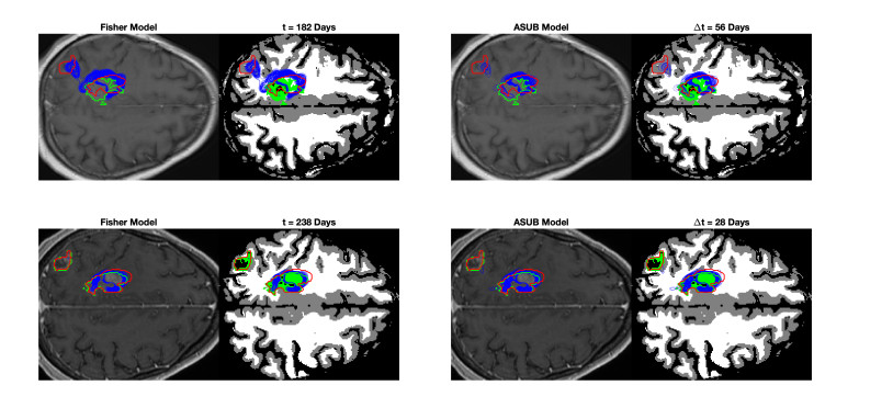
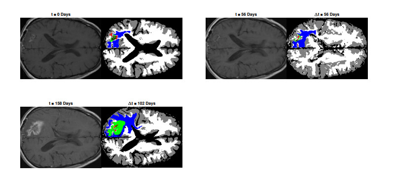
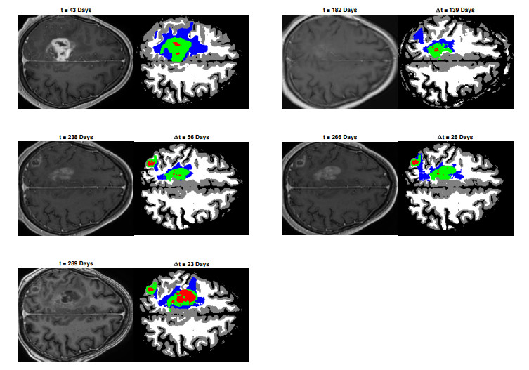
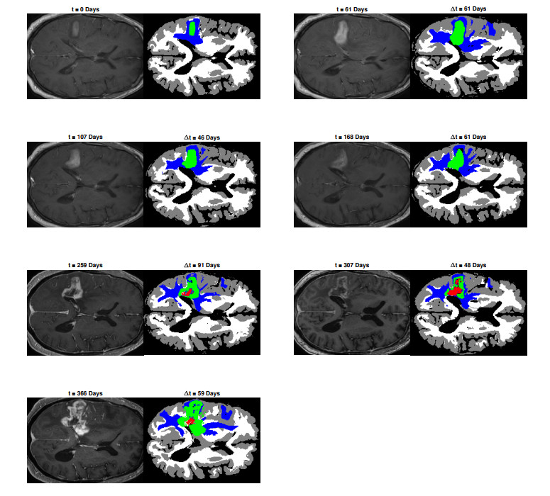
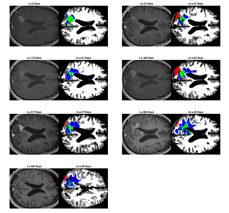
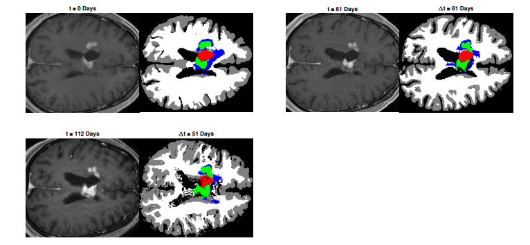
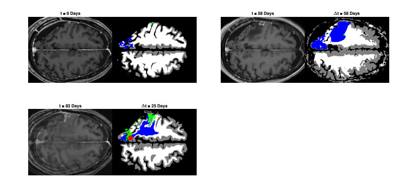
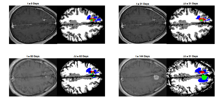
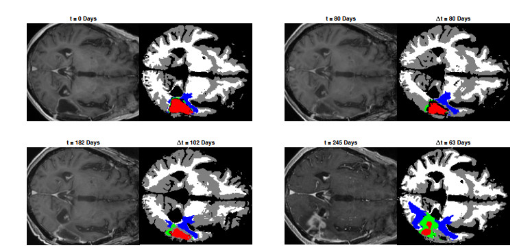
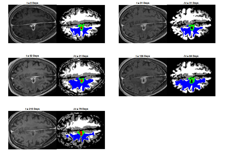
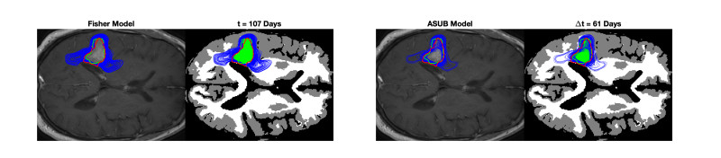
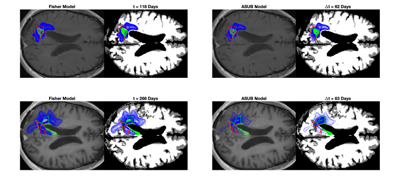
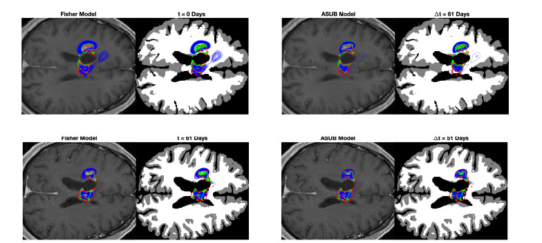
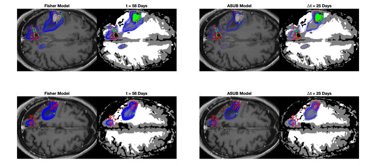
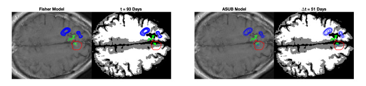
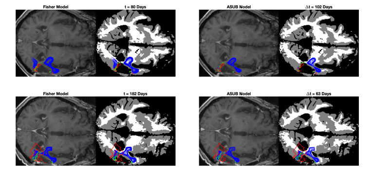
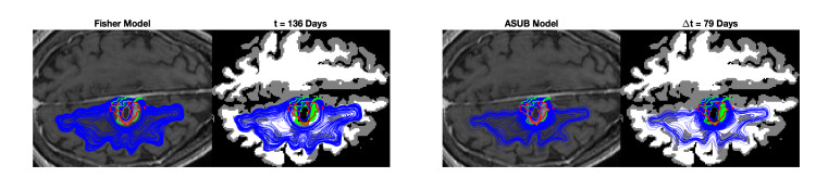
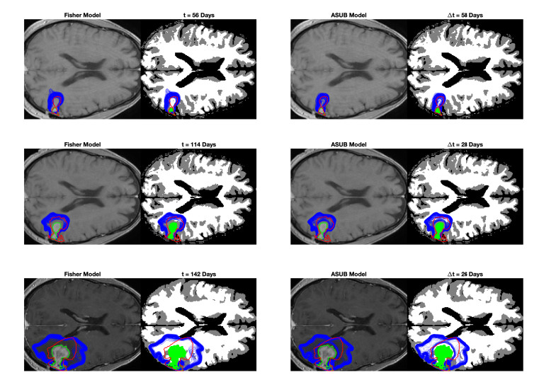
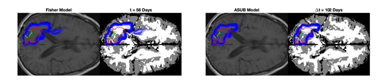
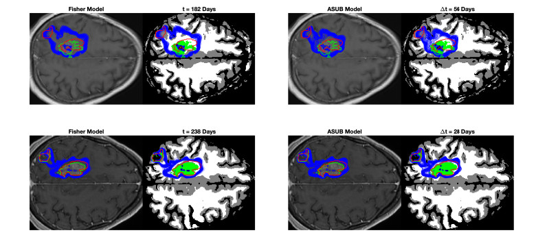
We describe a preliminary effort to model the growth and progression of glioblastoma multiforme, an aggressive form of primary brain cancer, in patients undergoing treatment for recurrence of tumor following initial surgery and chemoradiation. Two reaction-diffusion models are used: the Fisher-Kolmogorov equation and a 2-population model, developed by the authors, that divides the tumor into actively proliferating and quiescent (or necrotic) cells. The models are simulated on 3-dimensional brain geometries derived from magnetic resonance imaging (MRI) scans provided by the Barrow Neurological Institute. The study consists of 17 clinical time intervals across 10 patients that have been followed in detail, each of whom shows significant progression of tumor over a period of 1 to 3 months on sequential follow up scans. A Taguchi sampling design is implemented to estimate the variability of the predicted tumors to using $ 144 $ different choices of model parameters. In $ 9 $ cases, model parameters can be identified such that the simulated tumor, using both models, contains at least 40 percent of the volume of the observed tumor. We discuss some potential improvements that can be made to the parameterizations of the models and their initialization.
- Fisher-Kolmogorov model,
- glioblastoma multiforme,
- ensemble prediction,
- parameter estimation,
- magnetic resonance imaging,
- reaction-diffusion equations
Citation: Duane C. Harris, Giancarlo Mignucci-Jiménez, Yuan Xu, Steffen E. Eikenberry, C. Chad Quarles, Mark C. Preul, Yang Kuang, Eric J. Kostelich. Tracking glioblastoma progression after initial resection with minimal reaction-diffusion models[J]. Mathematical Biosciences and Engineering, 2022, 19(6): 5446-5481. doi: 10.3934/mbe.2022256

Related Papers:

Abstract

We describe a preliminary effort to model the growth and progression of glioblastoma multiforme, an aggressive form of primary brain cancer, in patients undergoing treatment for recurrence of tumor following initial surgery and chemoradiation. Two reaction-diffusion models are used: the Fisher-Kolmogorov equation and a 2-population model, developed by the authors, that divides the tumor into actively proliferating and quiescent (or necrotic) cells. The models are simulated on 3-dimensional brain geometries derived from magnetic resonance imaging (MRI) scans provided by the Barrow Neurological Institute. The study consists of 17 clinical time intervals across 10 patients that have been followed in detail, each of whom shows significant progression of tumor over a period of 1 to 3 months on sequential follow up scans. A Taguchi sampling design is implemented to estimate the variability of the predicted tumors to using $ 144 $ different choices of model parameters. In $ 9 $ cases, model parameters can be identified such that the simulated tumor, using both models, contains at least 40 percent of the volume of the observed tumor. We discuss some potential improvements that can be made to the parameterizations of the models and their initialization.

References

[1]	I. W. Pan, S. D. Ferguson, S. Lam, Patient and treatment factors associated with survival among adult glioblastoma patients: A USA population-based study from 2000–2010, J. Clin. Neurosci., 22 (2015), 1575–1581. https://doi.org/10.1016/j.jocn.2015.03.032 doi: 10.1016/j.jocn.2015.03.032
[2]	R. Stupp, W. P. Mason, M. J. Van Den Bent, M. Weller, B. Fisher, M. J. B. Taphoorn, et al., Radiotherapy plus concomitant and adjuvant temozolomide for glioblastoma, New Engl. J. Med., 352 (2005), 987–996. https://doi.org/10.1056/NEJMoa043330 doi: 10.1056/NEJMoa043330
[3]	M. Eriksson, J. Kahari, A. Vestman, M. Hallmans, M. Johansson, A. T. Bergenheim, et al., Improved treatment of glioblastoma–changes in survival over two decades at a single regional Centre. Acta Oncol., 58 (2019), 334–341. https://doi.org/10.1080/0284186X.2019.1571278
[4]	M. Weller, T. Cloughesy, J. R. Perry, W. Wick, Standards of care for treatment of recurrent glioblastoma–-are we there yet?, Neuro-Oncology, 15 (2013), 4–27. https://doi.org/10.1093/neuonc/nos273 doi: 10.1093/neuonc/nos273
[5]	K. Seystahl, W. Wick, M. Weller, Therapeutic options in recurrent glioblastoma–an update, Crit. Rev. Oncol. Hemat., 99 (2016), 389–408. https://doi.org/10.1016/j.critrevonc.2016.01.018 doi: 10.1016/j.critrevonc.2016.01.018
[6]	C. Fernandes, A. Costa, L. Osório, R. C. Lago, P. Linhares, B. Carvalho, et al., Current Standards of Care in Glioblastoma Therapy, in Glioblastoma [Internet] (ed. S. De Vleeschouwer), Codon Publications, Brisbane (AU), 2017. https://doi.org/10.15586/codon.glioblastoma.2017.ch11
[7]	S. Lowe, K. P. Bhat, A. Olar, Current clinical management of patients with glioblastoma. Cancer Rep., 2 (2019), e1216. https://doi.org/10.1002/cnr2.1216
[8]	C. Birzu, P. French, M. Caccese, G. Cerretti, A. Idbaih, V. Zagonel, et al., Recurrent Glioblastoma: From Molecular Landscape to New Treatment Perspectives, Cancers, 13 (2021), 47. https://doi.org/10.3390/cancers13010047 doi: 10.3390/cancers13010047
[9]	E. Audureau, A. Chivet, R. Ursu, R. Corns, P. Metellus, G. Noel, et al., Prognostic factors for survival in adult patients with recurrent glioblastoma: A decision-tree-based model, J. Neuro-Oncol., 136 (2018), 565–576. https://doi.org/10.1007/s11060-017-2685-4 doi: 10.1007/s11060-017-2685-4
[10]	C. McBain, T. A. Lawrie, E. Rogozińska, A. Kernohan, T. Robinson, S. Jefferies, Treatment options for progression or recurrence of glioblastoma: A network meta-analysis. Cochrane DB. Syst. Rev. 2021, 1 (2021), CD013579. https://doi.org/10.1002/14651858.CD013579.pub2
[11]	R. Stupp, S. Taillibert, A. Kanner, W. Read, D. M. Steinberg, B. Lhermitte, et al., Effect of tumor-treating fields plus maintenance temozolomide vs maintenance temozolomide alone on survival in patients with glioblastoma: a randomized clinical trial, JAMA, 318 (2017), 2306–2316. https://doi.org/10.1001/jama.2017.18718 doi: 10.1001/jama.2017.18718
[12]	O. Rominiyi, A. Vanderlinden, S. J. Clenton, C. Bridgewater, Y. Al-Tamimi, S. J. Collis, Tumor treating fields therapy for glioblastoma: Current advances and future directions, Brit. J. Cancer, 124 (2021), 697–709. https://doi.org/10.1038/s41416-020-01136-5 doi: 10.1038/s41416-020-01136-5
[13]	D. Yang, Standardized MRI assessment of high-grade glioma response: A review of the essential elements and pitfalls of the RANO criteria. Neuro-Oncol. Pract., 3 (2016), 59–67. https://doi.org/10.1093/nop/npv023
[14]	O. Eidel, S. Burth, J. O. Neumann, P. J. Kieslich, F. Sahm, C. Jungk, et al., Tumor infiltration in enhancing and non-enhancing parts of glioblastoma: A correlation with histopathology, PLOS ONE, 12 (2017), e0169292. https://doi.org/10.1371/journal.pone.0169292 doi: 10.1371/journal.pone.0169292
[15]	J. D. Murray, Mathematical Biology, 3$^{rd}$ Edition, Springer-Verlag, 2003. https://doi.org/10.1007/b98869
[16]	R. A. Fisher, The wave of advance of advantageous genes, Ann. Eugen., 7 (1937), 355–369. https://doi.org/10.1111/j.1469-1809.1937.tb02153.x doi: 10.1111/j.1469-1809.1937.tb02153.x
[17]	O. Clatz, M. Sermesant, P. Y. Bondiau, H. Delingette, S. K. Warfield, G. Malandain, et al., Realistic simulation of the 3-D growth of brain tumors in MR images coupling diffusion with biomechanical deformation, IEEE T. Med. Imaging, 24 (2005), 1334–1346. https://doi.org/10.1109/TMI.2005.857217 doi: 10.1109/TMI.2005.857217
[18]	C. Hogea, C. Davatzikos, G. Biros, An image-driven parameter estimation problem for a reaction–diffusion glioma growth model with mass effects, J. Math. Biol., 56 (2008), 793-825. https://doi.org/10.1007/s00285-007-0139-x doi: 10.1007/s00285-007-0139-x
[19]	M. Lê, H. Delingette, J. Kalpathy-Cramer, E. R. Gerstner, T. Batchelor, J. Unkelbach, et al., Bayesian Personalization of Brain Tumor Growth Model, in Medical Image Computing and Computer-Assisted Intervention – MICCAI 2015 (eds. N. Navab, J. Hornegger, W. Wells, A. Frangi), MICCAI (2015), Lecture Notes in Computer Science, vol 9350, Springer, Cham. https://doi.org/10.1007/978-3-319-24571-3_51
[20]	D. A. Hormuth, K. A. Al Feghali, A. M. Elliott, T. E. Yankeelov, C. Chung, Image-based personalization of computational models for predicting response of high-grade glioma to chemoradiation, Sci. Rep., 11 (2021), 8520. https://doi.org/10.1038/s41598-021-87887-4 doi: 10.1038/s41598-021-87887-4
[21]	C. Martens, A. Rovai, D. Bonatto, T. Metens, O. Debeir, C. Decaestecker, et al., Deep Learning for Reaction-Diffusion Glioma Growth Modelling: Towards a Fully Personalized Model?, arXiv: 2111.13404, (2021). https://doi.org/10.48550/arXiv.2111.13404
[22]	E. Konukoglu, O. Clatz, B. H. Menze, B. Stieltjes, M. Weber, E. Mandonnet, H. Delingette, N. Ayache, Image Guided Personalization of Reaction-Diffusion Type Tumor Growth Models Using Modified Anisotropic Eikonal Equations, IEEE T. Med. Imag., 29 (2010), 77–95. https://doi.org/10.1109/TMI.2009.2026413 doi: 10.1109/TMI.2009.2026413
[23]	I. Rekik, S. Allassonnière, O. Clatz, E. Geremia, E. Stretton, H. Delingette, et al., Tumor growth parameters estimation and source localization from a unique time point: Application to low-grade gliomas, Comput. Vis. Image Und., 117 (2013), 238–249, https://doi.org/10.1016/j.cviu.2012.11.001 doi: 10.1016/j.cviu.2012.11.001
[24]	K. R. Swanson, R. C. Rostomily, E. C. Alvord Jr, A mathematical modelling tool for predicting survival of individual patients following resection of glioblastoma: a proof of principle, Brit. J. Cancer, 98 (2008), 113–119. https://doi.org/10.1038/sj.bjc.6604125 doi: 10.1038/sj.bjc.6604125
[25]	J. D. Murray, Glioblastoma brain tumours: Estimating the time from brain tumour initiation and resolution of a patient survival anomaly after similar treatment protocols, J. Biol. Dynam., 6 (2012), 118–127. https://doi.org/10.1080/17513758.2012.678392 doi: 10.1080/17513758.2012.678392
[26]	J. Lipková, P. Angelikopoulos, S. Wu, E. Alberts, B. Wiestler, C. Diehl, et al., Personalized Radiotherapy Design for Glioblastoma: Integrating Mathematical Tumor Models, Multimodal Scans, and Bayesian Inference, IEEE T. Med. Imaging, 38 (2019), 1875–1884. https://doi.org/10.1109/TMI.2019.2902044 doi: 10.1109/TMI.2019.2902044
[27]	T. C. Steed, J. M. Treiber, M. G. Brandel, A. Fotopoulos, S. Voulgaris, M. I. Argyropoulou, Quantification of glioblastoma mass effect by lateral ventricle displacement Sci. Rep., 8 (2018), 2827. https://doi.org/10.1038/s41598-018-21147-w
[28]	A. Zikou, C. Sioka, G. A. Alexiou, A. Fotopoulos, S. Voulgaris, M. I. Argyropoulou, Radiation Necrosis, Pseudoprogression, Pseudoresponse, and Tumor Recurrence: Imaging Challenges for the Evaluation of Treated Gliomas, Contrast Media Mol. I., 2018 (2018), 6828396. https://doi.org/10.1155/2018/6828396 doi: 10.1155/2018/6828396
[29]	O. D. Arevalo, C. Soto, P. Reblei, A. Kamali, L. Y. Ballester, Y. Esquenazi, et al., Assessment of glioblastoma response in the era of bevacizumab: Longstanding and emergent challenges in the imaging evaluation of pseudoresponse, Front. Neurol., 10 (2019), 460. https://doi.org/10.3389/fneur.2019.00460 doi: 10.3389/fneur.2019.00460
[30]	J. A. Sherratt, Wavefront propagation in a competition equation with a new motility term modelling contact inhibition between cell populations, Proc. R. Soc. Lond. A., 456 (2000), 2365-–2386. https://doi.org/10.1098/rspa.2000.0616 doi: 10.1098/rspa.2000.0616
[31]	J. A. Sherratt, M. A. Chaplain, A new mathematical model for avascular tumour growth, J. Math. Biol., 43 (2001), 291–312. https://doi.org/10.1007/s002850100088 doi: 10.1007/s002850100088
[32]	K. R. Swanson, R. C. Rockne, J. Claridge, M. A. Chaplain, E. C. Alvord Jr, R. A. Alexander, et al., Quantifying the Role of Angiogenesis in Malignant Progression of Gliomas: In Silico Modeling Integrates Imaging and Histology, Cancer Res., 71 (2011), 7366–7375. https://doi.org/10.1088/0031-9155/57/1/225 doi: 10.1088/0031-9155/57/1/225
[33]	T. L. Stepien, E. M. Rutter, Y. Kuang, Traveling waves of a go-or-grow model of glioma growth, SIAM J. Appl. Math., 78 (2018), 1778–1801. https://doi.org/10.1137/17M1146257 doi: 10.1137/17M1146257
[34]	L. Han, S. Eikenberry, C. He, L. Johnson, M. C. Preul, E. J. Kostelich, Y. Kuang, Patient-specific parameter estimates of glioblastoma multiforme growth dynamics from a model with explicit birth and death rates, Math. Biosci. Eng., 16 (2019), 5307–5323. https://doi.org/10.3934/mbe.2019265 doi: 10.3934/mbe.2019265
[35]	Y. Kuang, J. D. Nagy, S. E. Eikenberry, Introduction to Mathematical Oncology, 1$^{st}$ edition, Chapman and Hall/CRC, 2016. https://doi.org/10.1201/9781315365404
[36]	R. S Rao, C. G. Kumar, R. S. Prakasham, P. J. Hobbs, The Taguchi methodology as a statistical tool for biotechnological applications: A critical appraisal, Biotechnol. J., 3 (2008), 510–523. https://doi.org/10.1002/biot.200700201 doi: 10.1002/biot.200700201
[37]	W. D. Penny, K. J. Friston, J. T. Ashburner, S. J. Kiebel, T. E. Nichols, Statistical Parametric Mapping: The analysis of Functional Brain Images, 1$^{st}$ edition, Academic Press, London, 2007. https://doi.org/10.1016/B978-0-12-372560-8.X5000-1
[38]	A. Fedorov, R. Beichel, J. Kalpathy-Cramer, J. Finet, J. C. Fillion-Robin, S. Pujol, et al., 3D Slicer as an image computing platform for the Quantitative Imaging Network, Magn. Reson. Imaging, 30 (2012), 1323–1341. https://doi.org/10.1016/j.mri.2012.05.001 doi: 10.1016/j.mri.2012.05.001
[39]	P. D. Chang, H. R. Malone, S. G. Bowden, D. S. Chow, B. J. A. Gill, T. H. Ung, et al., A multiparametric model for mapping cellularity in glioblastoma using radiographically localized biopsies, Am. J. Neuroradiol., 38 (2017), 890–898. https://doi.org/10.3174/ajnr.A5112 doi: 10.3174/ajnr.A5112
[40]	E. Gates, J. S. Weinberg, S. S. Prabhu, J. S. Lin, J. Hamilton, J. D. Hazle, et al., Estimating local cellular density in glioma using MR imaging data, Am. J. Neuroradiol., 42 (2021), 102–108. https://doi.org/10.3174/ajnr.A6884 doi: 10.3174/ajnr.A6884
[41]	L. F. Shampine, B. P. Sommeijer, J. G. Verwer, IRKC: An IMEX solver for stiff diffusion–reaction PDEs, J. Comput. Appl. Math., 196 (2006), 485–497. https://doi.org/10.1016/j.cam.2005.09.014 doi: 10.1016/j.cam.2005.09.014
[42]	M. Dowle, R. M. Mantel, D. Barkley, Fast simulations of waves in three-dimensional excitable media, Int. J. Bifurcat. Chaos, 7 (1997), 2529–-2545. https://doi.org/10.1142/S0218127497001692 doi: 10.1142/S0218127497001692
[43]	H. Akaike, A new look at the statistical model identification, IEEE T. Automat. Contr., 19 (1974), 716-723. https://doi.org/10.1109/TAC.1974.1100705 doi: 10.1109/TAC.1974.1100705
[44]	Z. X. Lin, Glioma-related edema: New insight into molecular mechanisms and their clinical implications, Chin. J. Cancer, 32 (2013), 49–52. https://doi.org/10.5732/cjc.012.10242 doi: 10.5732/cjc.012.10242
[45]	X. Qin, R. Liu, F. Akter, L. Qin, Q. Xie, Y. Li, et al., Peri-tumoral brain edema associated with glioblastoma correlates with tumor recurrence, J. Cancer, 12 (2021), 2073–2082. https://doi.org/10.7150/jca.53198 doi: 10.7150/jca.53198
[46]	M. Cenciarini, M. Valentino, S. Belia, L. Sforna, P. Rosa, S. Ronchetti, et al., Dexamethasone in glioblastoma multiforme therapy: Mechanisms and controversies, Front. Mol. Neurosc., 12 (2019). https://doi.org/10.3389/fnmol.2019.00065
[47]	E. J. Kostelich, Y. Kuang, J. M. McDaniel, N. Z. Moore, N. L. Martirosyan, et al., Accurate state estimation from uncertain data and models: An application of data assimilation to mathematical models of human brain tumors, Biol. Direct, 6 (2011), 64. https://doi.org/10.1186/1745-6150-6-64 doi: 10.1186/1745-6150-6-64
[48]	J. McDaniel, E. Kostelich, Y. Kuang, J. Nagy, M. C. Preul, N. Z. Moore, et al., Data Assimilation in Brain Tumor Models, in Mathematical Methods and Models in Biomedicine (eds. U. Ledzewicz, H. Schättler, A. Friedman, E. Kashdan), Springer, New York, NY, 2013,233–262. https://doi.org/10.1007/978-1-4614-4178-6_9

Reader Comments

Your name:*

Email:*
© 2022 the Author(s), licensee AIMS Press. This is an open access article distributed under the terms of the Creative Commons Attribution License (http://creativecommons.org/licenses/by/4.0)