Effects of dispersed fibres in myocardial mechanics, Part II: active response

Debao Guan; Yingjie Wang; Lijian Xu; Li Cai; Xiaoyu Luo; Hao Gao; Debao Guan; Yingjie Wang; Lijian Xu; Li Cai; Xiaoyu Luo; Hao Gao

doi:10.3934/mbe.2022189

Mathematical Biosciences and Engineering

2022, Volume 19, Issue 4: 4101-4119. doi: 10.3934/mbe.2022189

Previous Article Next Article

Research article Special Issues

Effects of dispersed fibres in myocardial mechanics, Part II: active response

1.
School of Mathematics and Statistics, University of Glasgow, UK
2.
Centre for Perceptual and Interactive Intelligence, The Chinese University of Hong Kong, Hong Kong, China
3.
School of Mathematics and Statistics, Northwestern Polytechnical University, Xi'an, China

Received: 25 November 2021 Revised: 24 January 2022 Accepted: 25 January 2022 Published: 16 February 2022

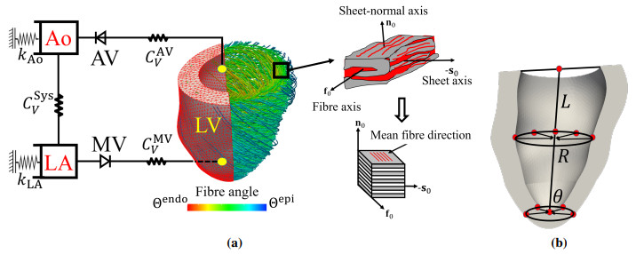
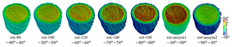
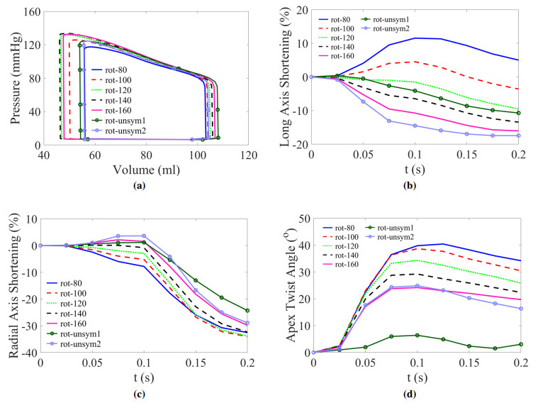
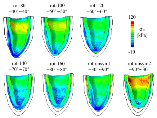
This work accompanies the first part of our study "effects of dispersed fibres in myocardial mechanics: Part I passive response" with a focus on myocardial active contraction. Existing studies have suggested that myofibre architecture plays an important role in myocardial active contraction. Following the first part of our study, we firstly study how the general fibre architecture affects ventricular pump function by varying the mean myofibre rotation angles, and then the impact of fibre dispersion along the myofibre direction on myocardial contraction in a left ventricle model. Dispersed active stress is described by a generalised structure tensor method for its computational efficiency. Our results show that both the myofibre rotation angle and its dispersion can significantly affect cardiac pump function by redistributing active tension circumferentially and longitudinally. For example, larger myofibre rotation angle and higher active tension along the sheet-normal direction can lead to much reduced end-systolic volume and higher longitudinal shortening, and thus a larger ejection fraction. In summary, these two studies together have demonstrated that it is necessary and essential to include realistic fibre structures (both fibre rotation angle and fibre dispersion) in personalised cardiac modelling for accurate myocardial dynamics prediction.
- fibre dispersion,
- myofibre rotation,
- generalised structure tensor,
- active stress,
- myocardial contraction
Citation: Debao Guan, Yingjie Wang, Lijian Xu, Li Cai, Xiaoyu Luo, Hao Gao. Effects of dispersed fibres in myocardial mechanics, Part II: active response[J]. Mathematical Biosciences and Engineering, 2022, 19(4): 4101-4119. doi: 10.3934/mbe.2022189

Related Papers:

Abstract

This work accompanies the first part of our study "effects of dispersed fibres in myocardial mechanics: Part I passive response" with a focus on myocardial active contraction. Existing studies have suggested that myofibre architecture plays an important role in myocardial active contraction. Following the first part of our study, we firstly study how the general fibre architecture affects ventricular pump function by varying the mean myofibre rotation angles, and then the impact of fibre dispersion along the myofibre direction on myocardial contraction in a left ventricle model. Dispersed active stress is described by a generalised structure tensor method for its computational efficiency. Our results show that both the myofibre rotation angle and its dispersion can significantly affect cardiac pump function by redistributing active tension circumferentially and longitudinally. For example, larger myofibre rotation angle and higher active tension along the sheet-normal direction can lead to much reduced end-systolic volume and higher longitudinal shortening, and thus a larger ejection fraction. In summary, these two studies together have demonstrated that it is necessary and essential to include realistic fibre structures (both fibre rotation angle and fibre dispersion) in personalised cardiac modelling for accurate myocardial dynamics prediction.

References

[1]	D. Guan, X. Zhuan, W. Holmes, X. Luo, H. Gao, Modelling of fibre dispersion and its effects on cardiac mechanics from diastole to systole, J. Eng. Math., 128 (2021), 1–24. https://doi.org/10.1007/s10665-021-10102-w doi: 10.1007/s10665-021-10102-w
[2]	K. Li, R. W. Ogden, G. A. Holzapfel, A discrete fibre dispersion method for excluding fibres under compression in the modelling of fibrous tissues, J. R. Soc. Interface, 15 (2018), 20170766. https://doi.org/10.1098/rsif.2017.0766 doi: 10.1098/rsif.2017.0766
[3]	T. C. Gasser, R. W. Ogden, G. A. Holzapfel, Hyperelastic modelling of arterial layers with distributed collagen fibre orientations, J. R. Soc. Interface, 3 (2006), 15–35. https://doi.org/10.1098/rsif.2005.0073 doi: 10.1098/rsif.2005.0073
[4]	G. A. Holzapfel, R. W. Ogden, S. Sherifova, On fibre dispersion modelling of soft biological tissues: a review, Proc. R. Soc. A, 475 (2019), 20180736. https://doi.org/10.1098/rspa.2018.0736 doi: 10.1098/rspa.2018.0736
[5]	D. Guan, Y. Mei, L. Xu, L. Cai, X. Luo, H. Gao, Effects of dispersed fibres in myocardial mechanics, Part I: passive response, Math. Biosci. Eng., 19 (2022), 3972–3993. https://doi.org/10.3934/mbe.2022183 doi: 10.3934/mbe.2022183
[6]	K. Mangion, H. Gao, D. Husmeier, X. Luo, C. Berry, Advances in computational modelling for personalised medicine after myocardial infarction, Heart, 104 (2018), 550–557. https://doi.org/10.1136/heartjnl-2017-311449 doi: 10.1136/heartjnl-2017-311449
[7]	M. Peirlinck, F. S. Costabal, J. Yao, J. M. Guccione, S. Tripathy, Y. Wang, et al., Precision medicine in human heart modeling, Biomech. Model. Mechanobiol., (2021), 1–29. https://doi.org/10.1007/s10237-021-01421-z doi: 10.1007/s10237-021-01421-z
[8]	D. H. S. Lin, F. C. P. Yin, A multiaxial constitutive law for mammalian left ventricular myocardium in steady-state barium contracture or tetanus, J. Biomech. Eng., 120 (1998), 504–517. https://doi.org/10.1115/1.2798021 doi: 10.1115/1.2798021
[9]	J. F. Wenk, D. Klepach, L. C. Lee, Z. Zhang, L. Ge, E. E. Tseng, et al., First evidence of depressed contractility in the border zone of a human myocardial infarction, Ann. Thorac. Surg., 93 (2012), 1188–1193. https://doi.org/10.1016/j.athoracsur.2011.12.066 doi: 10.1016/j.athoracsur.2011.12.066
[10]	M. Genet, L. C. Lee, R. Nguyen, H. Haraldsson, G. Acevedo-Bolton, Z. Zhang, et al., Distribution of normal human left ventricular myofiber stress at end diastole and end systole: a target for in silico design of heart failure treatments, J. Appl. Physiol., 117 (2014), 142–152. https://doi.org/10.1152/japplphysiol.00255.2014 doi: 10.1152/japplphysiol.00255.2014
[11]	K. L. Sack, E. Aliotta, D. B. Ennis, J. S. Choy, G. S. Kassab, J. M. Guccione, et al., Construction and validation of subject-specific biventricular finite-element models of healthy and failing swine hearts from high-resolution dt-mri, Front. Physiol., 9 (2018). https://doi.org/10.3389/fphys.2018.00539 doi: 10.3389/fphys.2018.00539
[12]	D. Guan, J. Yao, X. Luo, H. Gao, Effect of myofibre architecture on ventricular pump function by using a neonatal porcine heart model: from dt-mri to rule-based methods, R. Soc. Open Sci., 7 (2020), 191655. https://doi.org/10.1098/rsos.191655 doi: 10.1098/rsos.191655
[13]	T. S. E. Eriksson, A. J. Prassl, G. Plank, G. A. Holzapfel, Modeling the dispersion in electromechanically coupled myocardium, Int. J. Numer. Methods Biomed. Eng., 29 (2013), 1267–1284. https://doi.org/10.1002/cnm.2575 doi: 10.1002/cnm.2575
[14]	F. Ahmad, S. Soe, N. White, R. Johnston, I. Khan, J. Liao, et al., Region-specific microstructure in the neonatal ventricles of a porcine model, Ann. Biomed. Eng., 46 (2018), 2162–2176. https://doi.org/10.1007/s10439-018-2089-4 doi: 10.1007/s10439-018-2089-4
[15]	H. M. Wang, H. Gao, X. Y. Luo, C. Berry, B. E. Griffith, R. W. Ogden, et al., Structure-based finite strain modelling of the human left ventricle in diastole, Int. J. Numer. Methods Biomed. Eng., 29 (2013), 83–103. https://doi.org/10.1002/cnm.2497 doi: 10.1002/cnm.2497
[16]	B. Baillargeon, I. Costa, J. R. Leach, L. C. Lee, M. Genet, A. Toutain, et al., Human cardiac function simulator for the optimal design of a novel annuloplasty ring with a sub-valvular element for correction of ischemic mitral regurgitation, Cardiovasc. Eng. Technol., 6 (2015), 105–116. https://doi.org/10.1007/s13239-015-0216-z doi: 10.1007/s13239-015-0216-z
[17]	G. A. Holzapfel, J. A. Niestrawska, R. W. Ogden, A. J. Reinisch, A. J. Schriefl, Modelling non-symmetric collagen fibre dispersion in arterial walls, J. R. Soc. Interface, 12 (2015), 20150188. https://doi.org/10.1098/rsif.2015.0188 doi: 10.1098/rsif.2015.0188
[18]	J. M. Guccione, A. D. McCulloch, Mechanics of active contraction in cardiac muscle: Part I—constitutive relations for fiber stress that describe deactivation, J. Biomech. Eng., 115 (1993), 72–81. https://doi.org/10.1115/1.2895473 doi: 10.1115/1.2895473
[19]	H. Gao, A. Aderhold, K. Mangion, X. Luo, D. Husmeier, C. Berry, Changes and classification in myocardial contractile function in the left ventricle following acute myocardial infarction, J. R. Soc. Interface, 14 (2017), 20170203. https://doi.org/10.1098/rsif.2017.0203 doi: 10.1098/rsif.2017.0203
[20]	A. Documentation, U. Manual, Version 6.14-2, Dassault Systemes, 2014. Available from: http://130.149.89.49:2080/v6.14.
[21]	D. Guan, F. Liang, P. A. Gremaud, Comparison of the windkessel model and structured-tree model applied to prescribe outflow boundary conditions for a one-dimensional arterial tree model, J. Biomech., 49 (2016), 1583–1592. https://doi.org/10.1016/j.jbiomech.2016.03.037 doi: 10.1016/j.jbiomech.2016.03.037
[22]	H. Gao, W. G. Li, L. Cai, C. Berry, X. Y. Luo, Parameter estimation in a holzapfel–ogden law for healthy myocardium, J. Eng. Math., 95 (2015), 231–248. https://doi.org/10.1007/s10665-014-9740-3 doi: 10.1007/s10665-014-9740-3
[23]	D. Guan, X. Luo, H. Gao, Constitutive modelling of soft biological tissue from ex vivo to in vivo: myocardium as an example, in International Conference by Center for Mathematical Modeling and Data Science, Osaka University, Springer, (2020), 3–14. https://doi.org/10.1007/978-981-16-4866-3_1
[24]	H. Gao, H. Wang, C. Berry, X. Luo, B. E. Griffith, Quasi-static image-based immersed boundary-finite element model of left ventricle under diastolic loading, Int. J. Numer. Methods Biomed. Eng., 30 (2014), 1199–1222. https://doi.org/110.1002/cnm.2652 doi: 10.1002/cnm.2652
[25]	G. Sommer, A. J. Schriefl, M. Andrä, M. Sacherer, C. Viertler, H. Wolinski, et al., Biomechanical properties and microstructure of human ventricular myocardium, Acta Biomater., 24 (2015), 172–192. https://doi.org/10.1016/j.actbio.2015.06.031 doi: 10.1016/j.actbio.2015.06.031
[26]	G. M. Fomovsky, A. D. Rouillard, J. W. Holmes, Regional mechanics determine collagen fiber structure in healing myocardial infarcts, J. Mol. Cell. Cardiol., 52 (2012), 1083–1090. https://doi.org/10.1016/j.yjmcc.2012.02.012 doi: 10.1016/j.yjmcc.2012.02.012
[27]	W. W. Chen, H. Gao, X. Y. Luo, N. A. Hill, Study of cardiovascular function using a coupled left ventricle and systemic circulation model, J. Biomech., 49 (2016), 2445–2454. https://doi.org/10.1016/j.jbiomech.2016.03.009 doi: 10.1016/j.jbiomech.2016.03.009
[28]	Y. Wang, L. Cai, X. Feng, X. Luo, H. Gao, A ghost structure finite difference method for a fractional fitzhugh-nagumo monodomain model on moving irregular domain, J. Comput. Phys., 428 (2021), 110081. https://doi.org/10.1016/j.jcp.2020.110081 doi: 10.1016/j.jcp.2020.110081

Reader Comments

Your name:*

Email:*
© 2022 the Author(s), licensee AIMS Press. This is an open access article distributed under the terms of the Creative Commons Attribution License (http://creativecommons.org/licenses/by/4.0)