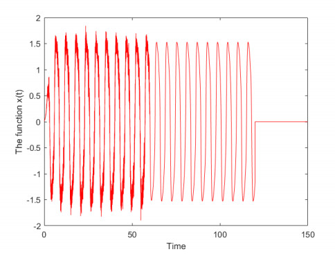
It has been noticed that heartbeats can display different patterns according to situations faced by a human. It has been indicated that, those passages from one pattern to another cannot be modelled using a single differential operator, either classical, fractional, or stochastic. In 2021, alternative concepts were introduced and called piecewise differentiation and integration, these concepts were applied in several complex problems with great insight. It is strongly believed that such will be leading concepts to modelling real-world problems with crossover behaviors. Crossover behaviors have been observed in heart rhythm, therefore, in this paper, the well-known van Der Pol equation will be subjected to piecewise analysis. Several simulations will be obtained using a numerical scheme based on Newton polynomial interpolation. Obtained figures show real world behaviors of heart rhythm with piecewise patterns.
Citation: Abdon Atangana, Seda İĞRET ARAZ. Rhythmic behaviors of the human heart with piecewise derivative[J]. Mathematical Biosciences and Engineering, 2022, 19(3): 3091-3109. doi: 10.3934/mbe.2022143
It has been noticed that heartbeats can display different patterns according to situations faced by a human. It has been indicated that, those passages from one pattern to another cannot be modelled using a single differential operator, either classical, fractional, or stochastic. In 2021, alternative concepts were introduced and called piecewise differentiation and integration, these concepts were applied in several complex problems with great insight. It is strongly believed that such will be leading concepts to modelling real-world problems with crossover behaviors. Crossover behaviors have been observed in heart rhythm, therefore, in this paper, the well-known van Der Pol equation will be subjected to piecewise analysis. Several simulations will be obtained using a numerical scheme based on Newton polynomial interpolation. Obtained figures show real world behaviors of heart rhythm with piecewise patterns.

| [1] | D. Baleanu, S. S. Sajjadi, A. Jajarmi, Ö. Defterli, J. H. Asad, The fractional dynamics of a linear triatomic molecule, Rom. Rep. Phys., 73 (2021), 1–13. |
| [2] |
A. Jajarmi, D. Baleanu, K. Z. Vahid, S. Mobayen, A general fractional formulation and tracking control for immunogenic tumor dynamics, Math. Methods Appl. Sci., 73 (2021). https://doi.org/10.1002/mma.7804 doi: 10.1002/mma.7804

|
| [3] | A. Atangana, S. Igret Araz, Deterministic-Stochastic modeling: A new direction in modeling real world problems with crossover effect, preprint, hal.archieves-ouverteshal-0320.1318. |
| [4] |
S. Nazari, A. Heydari, J. Khaligh, Modified modeling of the heart by applying nonlinear oscillators and designing proper control signal, Appl. Math., 4 (2013), 972–978. https://doi.org/10.4236/am.2013.47134 doi: 10.4236/am.2013.47134
|
| [5] |
A. Atangana, S. Igret Araz, Mathematical model of Covid-19 spread in Turkey and South Africa: Theory, methods and applications, Adv. Differ. Equ., 659 (2020). https://doi.org/10.1186/s13662-020-03095-w doi: 10.1186/s13662-020-03095-w
|
| [6] |
S. Igret Araz, Analysis of a Covid-19 model: Optimal control, stability and simulations Alexandria Eng. J., 60 (2020), 647–658. https://doi.org/10.1016/j.aej.2020.09.058 doi: 10.1016/j.aej.2020.09.058
|
| [7] |
A. Khan, R. Zarin, I Ahmed, A. Yusuf, U. W. Humphries, Numerical and theoretical analysis of Rabies model under the harmonic mean type incidence rate, Results Phys., 29 (2021), 104652. https://doi.org/10.1016/j.rinp.2021.104652 doi: 10.1016/j.rinp.2021.104652
|
| [8] |
D. Baleanu, S. S. Sajjadi, J. H. Asad, A. Jajarmi, E. Estiri, Hyperchaotic behaviors, optimal control, and synchronization of a nonautonomous cardiac conduction system, Adv. Differ. Equ., 157 (2021). https://doi.org/10.1186/s13662-021-03320-0 doi: 10.1186/s13662-021-03320-0
|
| [9] |
K. Göküs, M. Heinke, J. Hörth, Heart rhythm model for the simulation of electric fields in transesophageal atrial pacing and cardiac resynchronization therapy, Curr. Dir. Biomed. Eng., 4 (2018), 443–445. https://doi.org/10.1515/cdbme-2018-0105 doi: 10.1515/cdbme-2018-0105
|
| [10] |
M. Balakrishnan, V. S. Chakravarthy, S. Guhathakurta, Simulation of cardiac arrhythmias using a 2D heterogeneous whole heart model, Front. Physiol., 6 (2015), 374. https://doi.org/10.3389/fphys.2015.00374 doi: 10.3389/fphys.2015.00374
|
| [11] |
N. A. Trayanova, B. M. Tice, Integrative computational models of cardiac arrhythmias–simulating the structurally realistic heart, Drug Discov. Today Dis. Models, 6 (2009), 85–91. https://doi.org/10.1016/j.ddmod.2009.08.001 doi: 10.1016/j.ddmod.2009.08.001
|
| [12] |
J. Lian, H. Krätschmer, D. Müssig, Open Source Modeling of Heart Rhythm and Cardiac Pacing, Open Pacing Electrophysiol. Ther., 3 (2010), 28–44. https://doi.org/10.2174/1876536X01003010028 doi: 10.2174/1876536X01003010028
|
| [13] |
O. J. Peter, A. Yusuf, K. Oshinubi, F. A. Oguntolu, J. O. Lawal, A. I. Abioye, et. al., Fractional order of pneumococcal pneumonia infection model with Caputo Fabrizio operator, Results Phys. 29 (2021), 104581. https://doi.org/10.1016/j.rinp.2021.104581 doi: 10.1016/j.rinp.2021.104581
|
| [14] | D. Kaplan, L. Glass, Understanding nonlinear dynamics, Springer, (1995), 240–244. |
| [15] | G. M. V. Ladeira, G. V. Lima, J. M. Balthazar, A. M. Tusset, A. M.Bueno, P and T waves heart modeling with Van Der Pol Oscillator, 24th ABCM International Congress of Mechanical Engineering, (2017), Brazil. https://doi.org/10.26678/ABCM.COBEM2017.COB17-1151 |
| [16] | E. Ryzhii, M. Ryzhii, Modeling of Heartbeat Dynamics with a System of Coupled Nonlinear Oscillators, Commun. Comput. Inf. Sci., 404 (2014), 67–75. |
| [17] |
D. D. Bernardo, M. G. Signorini, S. Cerutti, A model of two nonlinear coupled oscillators for the study of heartbeat dynamics, Int. J. Bifurc. Chaos, 8 (1998), 1975–1985. https://doi.org/10.1142/S0218127498001637 doi: 10.1142/S0218127498001637
|
| [18] |
M. Caputo, M. Fabrizio, A new definition of fractional derivative without singular kernel, Prog. Fract. Differ. Appl., 1 (2015), 73–85. https://doi.org/10.12785/pfda/010201 doi: 10.12785/pfda/010201
|
| [19] |
A. Atangana, D. Baleanu, New fractional derivatives with non-local and non-singular kernel: Theory and application to heat transfer model, Therm. Sci., 20 (2016), 763–769. https://doi.org/10.98/TSCI160111018A doi: 10.98/TSCI160111018A
|
| [20] |
A Atangana, S. Igret Araz, Modeling third waves of Covid-19 spread with piecewise differential and integral operators: Turkey, Spain and Czechia, Results Phys., 20 (2021), 104694. https://doi.org/10.1016/j.rinp.2021.104694 doi: 10.1016/j.rinp.2021.104694
|
| [21] |
A. Atangana, S. Igret Araz, New concept in calculus: Piecewise differential and integral operators, Chaos Solit. Fract., 145 (2021), 110638. https://doi.org/10.1016/j.chaos.2020.110638 doi: 10.1016/j.chaos.2020.110638
|
| [22] |
A. Atangana, S. Igret Araz, New numerical scheme with Newton polynomial: Theory, Methods and Applications, Academic Press, (2021). https://doi.org/10.1016/B978-0-12-775850-3.50017-0 doi: 10.1016/B978-0-12-775850-3.50017-0
|


Figures(12)

Abdon Atangana, Seda İĞRET ARAZ. Rhythmic behaviors of the human heart with piecewise derivative[J]. Mathematical Biosciences and Engineering, 2022, 19(3): 3091-3109. doi: 10.3934/mbe.2022143


 DownLoad: