To overcome the two class imbalance problem among breast cancer diagnosis, a hybrid method by combining principal component analysis (PCA) and boosted C5.0 decision tree algorithm with penalty factor is proposed to address this issue. PCA is used to reduce the dimension of feature subset. The boosted C5.0 decision tree algorithm is utilized as an ensemble classifier for classification. Penalty factor is used to optimize the classification result. To demonstrate the efficiency of the proposed method, it is implemented on biased-representative breast cancer datasets from the University of California Irvine(UCI) machine learning repository. Given the experimental results and further analysis, our proposal is a promising method for breast cancer and can be used as an alternative method in class imbalance learning. Indeed, we observe that the feature extraction process has helped us improve diagnostic accuracy. We also demonstrate that the extracted features considering breast cancer issues are essential to high diagnostic accuracy.
Citation: Jian-xue Tian, Jue Zhang. Breast cancer diagnosis using feature extraction and boosted C5.0 decision tree algorithm with penalty factor[J]. Mathematical Biosciences and Engineering, 2022, 19(3): 2193-2205. doi: 10.3934/mbe.2022102
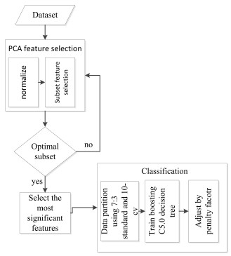
To overcome the two class imbalance problem among breast cancer diagnosis, a hybrid method by combining principal component analysis (PCA) and boosted C5.0 decision tree algorithm with penalty factor is proposed to address this issue. PCA is used to reduce the dimension of feature subset. The boosted C5.0 decision tree algorithm is utilized as an ensemble classifier for classification. Penalty factor is used to optimize the classification result. To demonstrate the efficiency of the proposed method, it is implemented on biased-representative breast cancer datasets from the University of California Irvine(UCI) machine learning repository. Given the experimental results and further analysis, our proposal is a promising method for breast cancer and can be used as an alternative method in class imbalance learning. Indeed, we observe that the feature extraction process has helped us improve diagnostic accuracy. We also demonstrate that the extracted features considering breast cancer issues are essential to high diagnostic accuracy.

| [1] |
L. A. Torre, F. Bray, R. L. Siegel, J. Ferlay, J. Lortet-Tieulent, A. Jemal, Global cancer statistics, 2012, CA Cancer J. Clin., 65 (2015), 87–108. https://doi.org/10.3322/caac.21262 doi: 10.3322/caac.21262

|
| [2] |
M. F. Akay, Support vector machines combined with feature selection for breast cancer diagnosis, Expert Syst. Appl., 36 (2009), 3240–3247. https://doi.org/10.1016/j.eswa.2008.01.009 doi: 10.1016/j.eswa.2008.01.009
|
| [3] |
R. L. Siegel, K. D. Miller, A. Jemal, Cancer statistics, 2018, CA Cancer J. Clin., 68 (2018), 7–30. https://doi.org/10.3322/caac.21442 doi: 10.3322/caac.21442
|
| [4] |
L. Peng, W. Chen, W. Zhou, F. Li, J. Yang, J. Zhang, An immune-inspired semi-supervised algorithm for breast cancer diagnosis, Comput. Methods Programs Biomed., 134 (2016), 259–265. https://doi.org/10.1016/j.cmpb.2016.07.020 doi: 10.1016/j.cmpb.2016.07.020
|
| [5] |
H. L. Chen, B. Yang, J. Liu, D. Y. Liu, A support vector machine classifier with rough set-based feature selection for breast cancer diagnosis, Expert Syst. Appl., 38 (2011), 9014–9022. https://doi.org/10.1016/j.eswa.2011.01.120 doi: 10.1016/j.eswa.2011.01.120
|
| [6] |
J. B. Li, Y. Peng, D. Liu, Quasiconformal kernel common locality discriminant analysis with application to breast cancer diagnosis, Inf. Sci., 223 (2013), 256–269. https://doi.org/10.1016/j.ins.2012.10.016 doi: 10.1016/j.ins.2012.10.016
|
| [7] |
B. Zheng, S. W. Yoon, S. S. Lam, Breast cancer diagnosis based on feature extraction using a hybrid of K-means and support vector machine algorithms, Expert Syst. Appl., 4 (2014), 1476–1482. https://doi.org/10.1016/j.eswa.2013.08.044 doi: 10.1016/j.eswa.2013.08.044
|
| [8] |
F. Gorunescu, S. Belciug, Evolutionary strategy to develop learning-based decision systems. Application to breast cancer and liver fibrosis stadialization, J. Biomed. Inform., 49 (2014), 112–118. https://doi.org/10.1016/j.jbi.2014.02.001 doi: 10.1016/j.jbi.2014.02.001
|
| [9] |
M. Karabatak, A new classifier for breast cancer detection based on Naive Bayesian, Meas., 72 (2015), 32–36. https://doi.org/10.1016/j.measurement.2015.04.028 doi: 10.1016/j.measurement.2015.04.028
|
| [10] |
R. Sheikhpour, M. A. Sarram, R. Sheikhpour, Particle swarm optimization for bandwidth determination and feature selection of kernel density estimation based classifiers in diagnosis of breast cancer, Appl. Soft Comput., 40 (2016), 113–131. https://doi.org/10.1016/j.asoc.2015.10.005 doi: 10.1016/j.asoc.2015.10.005
|
| [11] |
M. F. Ijaz, M. Attique, Y. Son, Data-driven cervical cancer prediction model with outlier detection and over-sampling methods, Sensors, 20 (2020), 2809. https://doi.org/10.3390/s20102809 doi: 10.3390/s20102809
|
| [12] |
M. Mandal, P. K. Singh, M. F. Ijaz, J. Shafi, R. Sarkar, A Tri-Stage Wrapper-Filter Feature Selection Framework for Disease Classification, Sensors, 21 (2021), 5571. https://doi.org/10.3390/s21165571 doi: 10.3390/s21165571
|
| [13] |
H. Patel, G. S. Thakur, Classification of imbalanced data using a modified fuzzy-neighbor weighted approach, Int. J. Intell. Eng. Syst., 10 (2017), 56–64. https://doi.org/10.22266/ijies2017.0228.07 doi: 10.22266/ijies2017.0228.07
|
| [14] |
W. C. Lin, C. F. Tsai, Y. H. Hu, J. S. Jhang, Clustering-based undersampling in class-imbalanced data, Inf. Sci., 409 (2017), 17–26. https://doi.org/10.1016/j.ins.2017.05.008 doi: 10.1016/j.ins.2017.05.008
|
| [15] |
P. D. Turney, Cost-sensitive classification: Empirical evaluation of a hybrid genetic decision tree induction algorithm, J. Artif. Intell. Res., 2 (1994), 369–409. https://doi.org/10.1613/jair.120 doi: 10.1613/jair.120
|
| [16] |
H. E. Kiziloz, Classifier ensemble methods in feature selection, Neurocomputing, 419 (2021), 97–107. https://doi.org/10.1016/j.neucom.2020.07.113 doi: 10.1016/j.neucom.2020.07.113
|
| [17] |
M. Galar, A. Fernández, E. Barrenechea, H. Bustince, F. Herrera, Ordering-based pruning for improving the performance of ensembles of classifiers in the framework of imbalanced datasets, Inf. Sci., 354 (2016), 178–196. https://doi.org/10.1016/j.ins.2016.02.056 doi: 10.1016/j.ins.2016.02.056
|
| [18] |
J. Zhang, L. Chen, J. Tian, F. Abid, W. Yang, X. Tang, Breast cancer diagnosis using cluster-based undersampling and boosted C5. 0 algorithm, Int. J. Control Autom. Syst., 19 (2021), 1998–2008. https://doi.org/10.1007/s12555-019-1061-x doi: 10.1007/s12555-019-1061-x
|
| [19] |
Z. Zheng, X. Wu, R. Srihari, Feature selection for text categorization on imbalanced data, ACM Sigkdd Explor. Newsl., 6 (2004), 80–89. https://doi.org/10.1145/1007730.1007741 doi: 10.1145/1007730.1007741
|
| [20] |
S. Punitha, F. Al-Turjman, T. Stephan, An automated breast cancer diagnosis using feature selection and parameter optimization in ANN, Comput. Electr. Eng., 90 (2021), 106958. https://doi.org/10.1016/j.compeleceng.2020.106958 doi: 10.1016/j.compeleceng.2020.106958
|
| [21] |
P. N. Srinivasu, J. G. SivaSai, M. F. Ijaz, A. K. Bhoi, W. Kim, J. J. Kang, Classification of skin disease using deep learning neural networks with MobileNet V2 and LSTM, Sensors, 21 (2021), 2852. https://doi.org/10.3390/s21082852 doi: 10.3390/s21082852
|
| [22] |
H. Naeem, A. A. Bin-Salem, A CNN-LSTM network with multi-level feature extraction-based approach for automated detection of coronavirus from CT scan and X-ray images, Appl. Soft Comput., 113 (2021), 107918. https://doi.org/10.1016/j.asoc.2021.107918 doi: 10.1016/j.asoc.2021.107918
|
| [23] |
P. Huang, Q. Ye, F. Zhang, G. Yang, W. Zhu, Z. Yang, Double L2, p-norm based PCA for feature extraction, Inf. Sci., 573 (2021), 345–359. https://doi.org/10.1016/j.ins.2021.05.079 doi: 10.1016/j.ins.2021.05.079
|
| [24] |
H. D. Cheng, X. J. Shi, R. Min, L. M. Hu, X. P. Cai, H. N. Du, Approaches for automated detection and classification of masses in mammograms, Pattern Recognit., 4 (2006), 646–668. https://doi.org/10.1016/j.patcog.2005.07.006 doi: 10.1016/j.patcog.2005.07.006
|
| [25] |
T. Raeder, G. Forman, N. V. Chawla, Learning from imbalanced data: Evaluation matters, in Data mining: Foundations and intelligent paradigms, Springer, (2012), 315–331. https://doi.org/10.1007/978-3-641-23166-7_12 doi: 10.1007/978-3-641-23166-7_12
|
| [26] |
S. Piri, D. Delen, T. Liu, A synthetic informative minority over-sampling (SIMO) algorithm leveraging support vector machine to enhance learning from imbalanced datasets, Decis. Support Syst., 106 (2018), 15–29. https://doi.org/10.1016/j.dss.2017.11.006 doi: 10.1016/j.dss.2017.11.006
|
| [27] |
C. Seiffert, T. M. Khoshgoftaar, J. Van. Hulse, A. Napolitano, RUSBoost: A hybrid approach to alleviating class imbalance, IEEE Trans. Syst. Man Cybern. Part A: Syst. Hum., 40 (2009), 185–197. https://doi.org/10.1109/tsmca.2009.2029559 doi: 10.1109/tsmca.2009.2029559
|
| [28] |
N. Liu, E. S. Qi, M. Xu, B. Gao, G. Q. Liu, A novel intelligent classification model for breast cancer diagnosis, Inf. Process. Manage., 56 (2019), 609–623. https://doi.org/10.1016/j.ipm.2018.10.014 doi: 10.1016/j.ipm.2018.10.014
|
| [29] |
S. Wang, Y. Wang, D. Wang, Y. Yin, Y. Wang, Y. Jin, An improved random forest-based rule extraction method for breast cancer diagnosis, Appl. Soft Comput., 86 (2020), 105941. https://doi.org/10.1016/j.asoc.2019.105941 doi: 10.1016/j.asoc.2019.105941
|
| [30] |
H. Wang, B. Zheng, S. W. Yoon, H. S. Ko, A support vector machine-based ensemble algorithm for breast cancer diagnosis, Eur. J. Oper. Res., 267 (Year), 687–699. https://doi.org/10.1016/j.ejor.2017.12.001 doi: 10.1016/j.ejor.2017.12.001
|
| [31] |
L. Breiman, Bagging predictors, Mach. Learn., 24 (1996), 123–140. https://doi.org/10.1007/BF00058655 doi: 10.1007/BF00058655
|
| [32] |
A. Taherkhani, G. Cosma, T. M. McGinnity, AdaBoost-CNN: An adaptive boosting algorithm for convolutional neural networks to classify multi-class imbalanced datasets using transfer learning, Neurocomputing, 404 (2020), 351–366. https://doi.org/10.1016/j.neucom.2020.03.064 doi: 10.1016/j.neucom.2020.03.064
|

Figures(2) / Tables(6)

Jian-xue Tian, Jue Zhang. Breast cancer diagnosis using feature extraction and boosted C5.0 decision tree algorithm with penalty factor[J]. Mathematical Biosciences and Engineering, 2022, 19(3): 2193-2205. doi: 10.3934/mbe.2022102


 DownLoad: