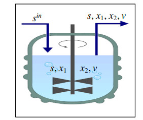
In this paper, we consider two species competing for a limiting substrate such that each species impedes the growth of the other one (Mutual inhibition) in presence of a virus inhibiting one bacterial species. A system of ordinary differential equations is proposed as a mathematical model for this competition. A detailed local qualitative analysis of the system is carried out. We proved that for a general nonlinear growth rates, the Competitive Exclusion Principle still valid, that at least one species goes extinct. For some cases where we have two locally stable equilibrium points, initial species concentrations are important in determining which is the winning species. Obtained results were confirmed by some numerical simulations using Matlab software.
Citation: Salah Alsahafi, Stephen Woodcock. Mutual inhibition in presence of a virus in continuous culture[J]. Mathematical Biosciences and Engineering, 2021, 18(4): 3258-3273. doi: 10.3934/mbe.2021162
In this paper, we consider two species competing for a limiting substrate such that each species impedes the growth of the other one (Mutual inhibition) in presence of a virus inhibiting one bacterial species. A system of ordinary differential equations is proposed as a mathematical model for this competition. A detailed local qualitative analysis of the system is carried out. We proved that for a general nonlinear growth rates, the Competitive Exclusion Principle still valid, that at least one species goes extinct. For some cases where we have two locally stable equilibrium points, initial species concentrations are important in determining which is the winning species. Obtained results were confirmed by some numerical simulations using Matlab software.

| [1] | H. L. Smith, P.Waltman, The theory of the chemostat, Dynamics of microbial competition, Cambridge Stud. Math. Biol., Cambridge Univ. Press, 1995. |
| [2] |
M. El Hajji, How can inter-specific interferences explain coexistence or confirm the competitive exclusion principle in a chemostat, Int. J. Biomath., 11 (2018), 1850111. doi: 10.1142/S1793524518501115

|
| [3] |
M. El Hajji, Modelling and optimal control for Chikungunya disease, Theory Biosci., 140 (2021), 27–44. doi: 10.1007/s12064-020-00324-4
|
| [4] |
G. Hardin, The competition exclusion principle, Science, 131 (1960), 1292–1298. doi: 10.1126/science.131.3409.1292
|
| [5] |
S. Hsu, S. Hubbell, P. Waltman, A mathematical theory for single-nutrient competition in continuous cultures of micro-organisms, SIAM J. Appl. Math., 32 (1977), 366. doi: 10.1137/0132030
|
| [6] |
G. J. Butler, G. S. K. Wolkowicz, A mathematical model of the chemostat with a general class of functions describing nutrient uptake, SIAM J. Appl. Math., 45 (1985), 138–151. doi: 10.1137/0145006
|
| [7] |
G. Wolkowicz, Z. Lu, Global dynamics of a mathematical model of competition in the chemostat: General response functions and differential death rates, SIAM J. Appl. Math., 52 (1992), 222–233. doi: 10.1137/0152012
|
| [8] | B. Li, Global asymptotic behavior of the chemostat: General response functions and different removal rates, SIAM J. Appl. Math., 59 (1999), 411–422. |
| [9] |
H. L. Smith, P. Waltman, Competition for a single limiting resource in continuous culture: The variable-yield model, SIAM J. Appl. Math., 54 (1994), 1113–1131. doi: 10.1137/S0036139993245344
|
| [10] |
S. R. Hansen, S. P. Hubbell, Single-nutrient microbial competition: Qualitative agreement between experimental and theoretically forecast outcomes, Science, 207 (1980), 1491–1493. doi: 10.1126/science.6767274
|
| [11] | A. Hurst, Nisin and other inhibitory substances from lactic acid bacteria, In Antimicrobials in Foods, ed. A. L. Branen $ & $ P. M. Davidson. Marcel Dekker, New York, (1983), 327–351. |
| [12] | A. Hurst, Nisin: Its preservative effect and function in the growth cycle of the producer organism, In Streptococci, ed. F. A. Skinner $ & $ L. B. Quesnel. Academic Press, London, (1978), 297–314. |
| [13] | A. A. Alderremy, M. Chamekh, F. Jeday, Semi-analytical solution for a system of competition with production a toxin in a chemostat, J. Math. Comput. SCI-JM. 20 (2020), 155–160. |
| [14] |
M. El Hajji, Boundedness and asymptotic stability of nonlinear Volterra integro-differential equations using Lyapunov functional, J. King Saud Univ. Sci., 31 (2019), 1516–1521. doi: 10.1016/j.jksus.2018.11.012
|
| [15] |
M. El Hajji, N. Chorfi, M. Jleli, Mathematical modelling and analysis for a three-tiered microbial food web in a chemostat, Electron. J. Diff. Eqns., 2017 (2017), 1–13. doi: 10.1186/s13662-016-1057-2
|
| [16] | M. El Hajji, N. Chorfi, M. Jleli, Mathematical model for a membrane bioreactor process, Electron, J. Diff. Eqns., 2015 (2015), 1–7. |
| [17] | M. El Hajji, J. Harmand, H. Chaker, C. Lobry, Association between competition and obligate mutualism in a chemostat, J. Biol. Dynamics. 3 (2009), 635–647. |
| [18] | M. El Hajji, S. Sayari, A. Zaghdani, Mathematical analysis of an "SIR" epidemic model in a continuous reactor–-deterministic and probabilistic approaches, J. Korean Math. Soc., 58 (2021), 45–67. |
| [19] | G. F. Gause, Experimental studies on the struggle for existence, J. Exp. Biol., 9 (1932), 389–402. |


Figures(6)

Salah Alsahafi, Stephen Woodcock. Mutual inhibition in presence of a virus in continuous culture[J]. Mathematical Biosciences and Engineering, 2021, 18(4): 3258-3273. doi: 10.3934/mbe.2021162


 DownLoad: