Global dynamics of a delayed alcoholism model with the effect of health education

Shuang Hong Ma; Hai Feng Huo; Hong Xiang; Shuang Lin Jing; Shuang Hong Ma; Hai Feng Huo; Hong Xiang; Shuang Lin Jing

doi:10.3934/mbe.2021048

Mathematical Biosciences and Engineering

2021, Volume 18, Issue 1: 904-932. doi: 10.3934/mbe.2021048

Previous Article Next Article

Research article Special Issues

Global dynamics of a delayed alcoholism model with the effect of health education

1.
Institute of Applied Mathematics, Lanzhou University of Technology, Lanzhou 730050, China
2.
College of Mathematical Sciences, Harbin Engineering University, Harbin 150001, China

Received: 06 October 2020 Accepted: 08 December 2020 Published: 04 January 2021

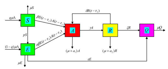
An alcohol consumption model with health education and three time delays is formulated and analyzed. The alcoholism generation number is defined. Two steady states of the model are found. At the same time, the corresponding global dynamics of the model are analyzed respectively in four cases with different time delays. Then, the effects of health education and three time delays in controlling the alcohol problem are discussed. Some numerical simulation results are also given to support our theoretical predictions.
- alcoholism model,
- time delays,
- health education,
- global dynamics,
- numerical simulation
Citation: Shuang Hong Ma, Hai Feng Huo, Hong Xiang, Shuang Lin Jing. Global dynamics of a delayed alcoholism model with the effect of health education[J]. Mathematical Biosciences and Engineering, 2021, 18(1): 904-932. doi: 10.3934/mbe.2021048

Related Papers:

Abstract

An alcohol consumption model with health education and three time delays is formulated and analyzed. The alcoholism generation number is defined. Two steady states of the model are found. At the same time, the corresponding global dynamics of the model are analyzed respectively in four cases with different time delays. Then, the effects of health education and three time delays in controlling the alcohol problem are discussed. Some numerical simulation results are also given to support our theoretical predictions.

References

[1]	F. S$\acute{a}$nchez, X. Wang, C. Castillo-Chávez, D. M. Gorman, P. J. Gruenewald, Drinking as an epidemic: a simple mathematical model with recovery and relapse, Therapists Guide to Evidence-Based Relapse Prevention, Academic Press, Burlington, (2007), 353–368.
[2]	J. Rehm, C. Mathers, S. Popova, M. Thavorncharoensap, Y. Teerawattananon, J. Patra, Global burden of disease and injury and economic cost attributable to alcohol use and alcohol-use disorders, Lancet, 373 (2009), 2223–2233. doi: 10.1016/S0140-6736(09)60746-7
[3]	J. Rehm, The risk associated with alcohol use and alcoholism, Alcohol Res. Health, 34 (2011), 135–143.
[4]	C. W. Lin, C. C. Lin, L. R. Moet, C. Y. Chang, D. S. Perng, C. C. Hsu, et al., Heavy alcohol consumption increases the incidence of hepatocellular carcinoma in hepatitis B virus-related cirrhosis, J. Hepatol., 58 (2013), 730–735. doi: 10.1016/j.jhep.2012.11.045
[5]	World Health Organization, Global Status Report on Alcohol and Health 2014, Geneva, Switzerland, 2014.
[6]	A. Corbern-Vallet, F. J. Santonja, M. Jornet-Sanz, R. J. Villanueva, Modeling chickenpox dynamics with a discrete time Bayesian stochastic compartmental model, Complexity, (2018), 1–9.
[7]	Q. Li, Z. Liu, S. Yuan, Cross-diffusion induced Turing instability for a competition model with saturation effect, Appl. Math. Compu., 347 (2019), 64–77.
[8]	D. Jia, T. Zhang, S. Yuan, Pattern dynamics of a diffusive doxin producing phytoplankton-zooplankton model with three-dimensional patch, Int. J. Bifurcation Chaos, 29 (2019), 1930011. doi: 10.1142/S0218127419300118
[9]	J. Yang, T. Zhang, S. Yuan, Turing pattern induced by cross-diffusion in a predator-prey model with pack predation-herd behavior, Int. J. Bifurcation Chaos, 30 (2020), 2050103. doi: 10.1142/S0218127420501035
[10]	X. Y. Meng, Y. Q. Wu, Dynamical analysis of a fuzzy phytoplankton Czooplankton model with refuge, fishery protection and harvesting, Appl. Math. Compu., 63 (2020), 361–389.
[11]	O. Sharomi, A. B. Gumel, Curtailing smoking dynamics: a mathematical modeling approach, Appl. Math. Compu., 195 (2008), 475–499.
[12]	H. F. Huo, C. C. Zhu, Influence of relapse in a giving up smoking model, Abstr. Appl. Anal., 2013 (2013), 1–12.
[13]	E. White, C. Comiskey, Heroin epidemics, treatment and ODE modelling, Math. Biosci., 208 (2007), 312–324.
[14]	G. Mulone, B. Straughan, A note on heroin epidemics, Math. Biosci., 218 (2009), 138–141. doi: 10.1016/j.mbs.2009.01.006
[15]	B. Benedict, Modelling alcoholism as a contagious disease: how "infected" drinking buddies spread problem drinking, SIAM News, 40 (2007), 1–3.
[16]	J. L. Manthey, A. Aidoob, K. Y. Ward, Campus drinking: an epidemiological model, J. Biol. Dyn., 2 (2008), 346–356. doi: 10.1080/17513750801911169
[17]	F. J. Santonja, E. Snchez, M. Rubio, J. Morera, Alcohol consumption in Spain and its economic cost: A mathematical modeling approach, Math. Comp. Model, 52 (2010), 999–1003. doi: 10.1016/j.mcm.2010.02.029
[18]	A. Mubayi, P. Greenwood, C. Castillo-Chavez, P. J. Gruenewald, D. M. Gorman, The impact of relative residence times on the distribution of heavy drinkers in highly distinct environments, Socio Econ. Plan Sci., 44 (2010), 45–56. doi: 10.1016/j.seps.2009.02.002
[19]	R. Bani, R. Hameed, S. Szymanowski, P. Greenwood, C. M. Kribs-Zaleta, A. Mubayi, Influence of environmental factors on college alcohol drinking patterns, Math. Biosci. Eng., 10 (2013), 1281–1300. doi: 10.3934/mbe.2013.10.1281
[20]	B. Buonomo, D. Lacitignola, Modeling peer influence effects on the spread of high Crisk alcohol consumption behavior, Ric. Mat., 63 (2014), 101–117. doi: 10.1007/s11587-013-0167-3
[21]	A. Mubayi, P. Greenwood, Contextual interventions for controlling alcohol drinking, Math. Popul. Stud., 20 (2013), 27–53. doi: 10.1080/08898480.2013.748588
[22]	G. Mulone, B. Straughan, Modeling binge drinking, Int. J. Biomath., 5 (2012), 1–14.
[23]	H. F. Huo, N. N. Song, Global stability for a binge drinking model with two stages, Discrete Dyn. Nat. Soc., 2012 (2012).
[24]	C. P. Bhunu, S. Mushayabasa, A theoretical analysis of smoking and alcoholism, J. Math. Model Algor., 11 (2012), 387–408. doi: 10.1007/s10852-012-9195-3
[25]	C. E. Walters, B. Straughan, R. Kendal, Modeling alcohol problems: total recovery, Ric. Mat., 62 (2013), 33–53. doi: 10.1007/s11587-012-0138-0
[26]	H. F. Huo, C. C. Zhu, Modeling the effect of constant immigration on drinking behaviour, J. Biol. Dyn., 11 (2017), 275–298. doi: 10.1080/17513758.2017.1337243
[27]	X. Y. Wang, H. F. Huo, Q. K. Kong, W. X. Shi, Optimal control strategies in an alcoholism model, Abstr. Appl. Anal., 2014 (2014).
[28]	S. Del Valle, A. M. Evangelista, M. C. Velasco, C. M. Kribs-Zaleta, S. H. Schmitz, Effects of education, vaccination and treatment on HIV transmission in homosexuals with genetic heterogeneity, Math. Biosci., 187 (2004), 111–133. doi: 10.1016/j.mbs.2003.11.004
[29]	R. Liu, J. Wu, H. Zhu, Media/psychological impact on multiple outbreaks of emerging infectious diseases, Comput. Math. Methods Med., 8 (2007), 153–164. doi: 10.1080/17486700701425870
[30]	F. Nayabadza, C. Chiyaka, Z. Mukandavire, S. D. Hove-musekma, Analysis of an HIV/AIDS mode with public health information campaigns and individual with drawal, J. Biol. Syst., 18 (2010), 357–375. doi: 10.1142/S0218339010003329
[31]	Y. Liu, J. Cui, The impact of media convergence on the dynamics of infectious diseases, Int. J. Biomath., 1 (2008), 65–74. doi: 10.1142/S1793524508000023
[32]	J. Cui, X. Tao, H. Zhu, An SIS infection model incorporating media coverage, Rocky Mt. J. Math, 38 (2008), 1323–1334.
[33]	J. Cui, Y. Sun, H. Zhu, The impact of media on the spreading and control of infectious diseases, J. Dyn. Diff. Eqns., 20 (2008), 31–53. doi: 10.1007/s10884-007-9075-0
[34]	C. Sun, W. Yang, J. Arino, K. Khan, Effect of mediainduced social distancing on disease transmission in a two patch setting, Math. Biosci., 230 (2011), 87–95. doi: 10.1016/j.mbs.2011.01.005
[35]	I. Z. Kiss, J. Cassell, M. Recker, P. L. Simon, The impact of information transmission on epidemic outbreaks, Math. Biosci., 255 (2010), 1–10.
[36]	S. Funk, E. Gilad, VAA. Jansen, Epidemic disease, awareness, and local behavioural response, J. Theor. Biol., 264 (2010), 501–509. doi: 10.1016/j.jtbi.2010.02.032
[37]	S. Samanta, S. Rana, A. Sharma, A. K. Misra, J. Chattopadhyay, Effects of awareness programs by media on the epidemic outbreaks: A mathematical model, Appl. Math. Comput., 219 (2013), 6965–6977.
[38]	Y. N. Xiao, T. T. Zhao, S. Y. Tang, Dynaamics of an infectious diseases with media/psychology induced non-smooth incidence, Math. Biosci. Eng., 10 (2013), 445–461. doi: 10.3934/mbe.2013.10.445
[39]	A. K. Misra, A. Sharma, J. B. Shukla, Modeling and analysis of effects of awareness programs by media on spread of infectious diseases, Math. Comp. Model, 53 (2011), 1221–1228. doi: 10.1016/j.mcm.2010.12.005
[40]	H. F. Huo, Q. Wang, Modeling the influence of awareness programs by media on the drinking dynamics, Abstr. Appl. Anal., 2014 (2014), 1–8.
[41]	H. Xiang, N. N. Song, H. F. Huo, Modelling effects of public health educational campaigns on drinking dynamics, J. Biol. Dyn., 10 (2015), 164–178.
[42]	S. H. Ma, H. F. Huo, H. Xiang, Threshold dynamics of a multi-group SEAR alcoholism model with public health education, Int. J. Biomath., 12 (2019), 39–62.
[43]	S. H. Ma, H. F. Huo, Global dynamics for a multi-group alcoholism model with public health education and alcoholism age, Math. Biosci. Eng., 16 (2019), 1683–1708. doi: 10.3934/mbe.2019080
[44]	A. K. Misra, A. Sharma, V. Singh, Effects of awareness programs in controlling the prevalence of an epidemic with time delay, J. Biol. Syst., 19 (2011), 389–402. doi: 10.1142/S0218339011004020
[45]	Y. Kuang, Delay Differential Equations with Applications in Population Dynamics, Academic Press, Boston, 1993.
[46]	J. Li, Y. Kuang, Analysis of model of the glucose-insulin regulatory system with two delays, SIAM J. Appl. Math., 67 (2007), 757–776. doi: 10.1137/050634001
[47]	J. Li, M. Wang, A. D. Gaetano, P. Palumbo, S. Panunzi, The range of time delay and the global stability of the equilibrium for an IVGTT model, Math. Biosci., 235 (2012), 128–137. doi: 10.1016/j.mbs.2011.11.005
[48]	C. Castillo-Chavez, B. Song, Dynamical models of tuberculosis and their applications, Math. Biosci. Eng., 1 (2004), 361–404. doi: 10.3934/mbe.2004.1.361
[49]	H. F. Huo, Y. L. Chen, H. Xiang, Stability of a binge drinking model with delay, J. Biol. Dyn., 11 (2017), 210–225. doi: 10.1080/17513758.2017.1301579
[50]	S. H. Ma, H. F. Huo, X. Y. Meng, Modelling alcoholism as a contagious cisease: a mathematical model with awareness programs and time delay, Discrete Dyn. Nat. Soc., 2015 (2015), 1–13.
[51]	P. V. Driessche, J. Watmough, Reproduction numbers and sub-threshold endemic equilibria for compartmental models of disease transmission, Math. Biosci., 180 (2002), 29–48. doi: 10.1016/S0025-5564(02)00108-6
[52]	H. H. Hyman, P. B. Shratsley, Some reasons why information campaigns fail, Pub. Opin. Quarl., 11 (1947), 412–423. doi: 10.1086/265867
[53]	M. Kot, Elements of Mathematical Biology, Cambridge University Press, Cambridge, 2001.
[54]	S. Ruan, J. Wei, On the zeros of transcendental functions with applications to stability of delay differential equations with two delays, Dyn. Contin. Discrete Impuls. Syst., Ser. A Math. Anal., 10 (2003), 863–874.
[55]	X. Li, J. Wei, On the zeros of a fourth degree exponential polynomial with applications to a neural network model with delays, Chaos, Solitons Fractals, 26 (2005), 519–526. doi: 10.1016/j.chaos.2005.01.019
[56]	M. D. Mckay, R. J. Beckman, W. J. Conover, Comparison of three methods for selecting values of input variables in the analysis of output from a computer code, Technometrics, 21 (1979), 239–245.
[57]	S. M. Blower, H. Dowlatabadi, Sensitivity and uncertainty analysis of complex models of disease transmission: an HIV model, as an example, Int. Stat. Rev., 62 (1994), 229–243. doi: 10.2307/1403510
[58]	S. Marino, I. B. Hogue, C. J. Ray, D. E. Kirschner, A methodology for performing global uncertainty and sensitivity analysis in systems biology, J. Theor. Biol., 254 (2008), 178–196. doi: 10.1016/j.jtbi.2008.04.011
[59]	F. Brauer, Compartmental Models in Epidemiology, Mathematical Epidemiology, Springer, Berlin, 2008, 19–79.
[60]	B. Sudret, Global sensitivity analysis using polynomial chaos expansions, Reliab. Eng. Sys. Saf., 93 (2008), 964–979. doi: 10.1016/j.ress.2007.04.002
[61]	J. Calatayud, B. M. Chen-Charpentier, J. C. López, M. J. Sanz, Combining polynomial chaos expansions and the random variable transformation technique to approximate the density function of stochastic problems, including some epidemiological models, Symmetry, 11 (2019), 43. doi: 10.3390/sym11010043
[62]	F. Santonja, B. M. Chen-Charpentier, Uncertainty quantification in simulations of epidemics using polynomial chaos, Comput. Math. Methods Med., 2012 2012.
[63]	J. Calatayud, M. Jornet, Mathematical modeling of adulthood obesity epidemic in Spain using deterministic, frequentist and Bayesian approaches, Chaos, Solitons Fractals, 140 (2020), 110179. doi: 10.1016/j.chaos.2020.110179
[64]	F. A. Dorini, R. Sampaio, Some results on the random wear coefficient of the archard model, J. Appl. Mech. 79 (2012), 051008.
[65]	F. J. Santonja, L. Shaikhet, Analysing social epidemics by delayed stochastic models, Discrete Dyn. Nat. Soc., 13 (2012), 1–13.
[66]	L. Shaikhet, Stability of some social mathematical models with delay under stochastic perturbations, Lyapunov Functionals and Stability of Stochastic Functional Differential Equations, Springer, Heidelberg, 2013,297–323.
[67]	F. J. Santonja, L. Shaikhet, Probabilistic stability analysis of social obesity epidemic by a delayed stochastic model, Nonlinear Anal.: Real World Appl., 17 (2014), 114–125. doi: 10.1016/j.nonrwa.2013.10.010

Reader Comments

Your name:*

Email:*
© 2021 the Author(s), licensee AIMS Press. This is an open access article distributed under the terms of the Creative Commons Attribution License (http://creativecommons.org/licenses/by/4.0)