Asymptotic behaviors of jellyfish model with stage structure

Zin Thu Win; Boping Tian; Shengqiang Liu; Zin Thu Win; Boping Tian; Shengqiang Liu

doi:10.3934/mbe.2021128

Mathematical Biosciences and Engineering

2021, Volume 18, Issue 3: 2508-2526. doi: 10.3934/mbe.2021128

Previous Article Next Article

Research article Special Issues

Asymptotic behaviors of jellyfish model with stage structure

1.
School of Mathematics, Harbin Institute of Technology, Harbin 150001, China
2.
School of Mathematical Sciences, Tiangong University, Tianjin 300387, China

Received: 31 August 2020 Accepted: 08 March 2021 Published: 15 March 2021

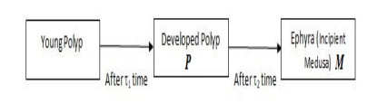
In this paper, a stage-structured jellyfish model with two time delays is formulated and analyzed, the first delay represents the time from the asexually reproduced young polyp to the mature polyp and the second denotes the time from the developed polyp to ephyra (incipient medusa). Global dynamics of the model are obtained via monotone dynamical theory: the jellyfish populations go extinct and the trivial equilibrium is globally asymptotically stable if the survival rate of polyp during cloning and the survival rate of the incipient medusa during strobilation are less than their death rates. And if the survival rate of polyp during cloning and the survival rate of the incipient medusa during strobilation are larger than their death rates, a unique positive equilibrium is globally asymptotically stable. Moreover, it is proved that the only stage of polyps will continue without growing into medusa and the boundary equilibrium is globally asymptotically stable if the survival rate of polyp is larger than its death rate during cloning and if there is no survival of the incipient medusa. Numerical simulations are performed to verify our analytical results and to explore the dynamics with/without delays.
- jellyfish,
- polyp-medusa,
- delay,
- global dynamics,
- stage structure
Citation: Zin Thu Win, Boping Tian, Shengqiang Liu. Asymptotic behaviors of jellyfish model with stage structure[J]. Mathematical Biosciences and Engineering, 2021, 18(3): 2508-2526. doi: 10.3934/mbe.2021128

Related Papers:

Abstract

In this paper, a stage-structured jellyfish model with two time delays is formulated and analyzed, the first delay represents the time from the asexually reproduced young polyp to the mature polyp and the second denotes the time from the developed polyp to ephyra (incipient medusa). Global dynamics of the model are obtained via monotone dynamical theory: the jellyfish populations go extinct and the trivial equilibrium is globally asymptotically stable if the survival rate of polyp during cloning and the survival rate of the incipient medusa during strobilation are less than their death rates. And if the survival rate of polyp during cloning and the survival rate of the incipient medusa during strobilation are larger than their death rates, a unique positive equilibrium is globally asymptotically stable. Moreover, it is proved that the only stage of polyps will continue without growing into medusa and the boundary equilibrium is globally asymptotically stable if the survival rate of polyp is larger than its death rate during cloning and if there is no survival of the incipient medusa. Numerical simulations are performed to verify our analytical results and to explore the dynamics with/without delays.

References

[1]	D. Pauly, W. Graham, S. Libralato, L. Morissette, M. D. Palomares, Jellyfish in ecosystems, online databases, and ecosystem models, Hydrobiologia, 616 (2009), 67–85. doi: 10.1007/s10750-008-9583-x
[2]	M. Grove, D. L. Breitburg, Growth and reproduction of gelatinous zooplankton exposed to low dissolved oxygen, Mar. Ecol. Prog. Ser., 301 (2005), 185–198. doi: 10.3354/meps301185
[3]	C. H. Han, S. I. Uye, Combined effects of food supply and temperature on asexual reproduction and somatic growth of polyps of the common jellyfish Aurelia aurita sl., Plankton Benthos Res., 5 (2010), 98–105. doi: 10.3800/pbr.5.98
[4]	Z. Dong, D. Liu, J. K. Keesing, Jellyfish blooms in China: Dominant species, causes and consequences, Mar. Pollut. Bull., 60 (2010), 954–963. doi: 10.1016/j.marpolbul.2010.04.022
[5]	E. Papathanassiou, P. Panayotidis, K. Anagnostaki, Notes on the biology and ecology of the jellyfish Aurelia aurita Lam. in Elefsis Bay (Saronikos Gulf, Greece), Mar. Ecol., 8 (1987), 49–58. doi: 10.1111/j.1439-0485.1987.tb00174.x
[6]	W. C. Liu, W. T. Lo, J. E. Purcell, H. H. Chang, Effects of temperature and light intensity on asexual reproduction of the scyphozoan, Aurelia aurita (L.) in Taiwan, Hydrobiologia, 616 (2009), 247–258. doi: 10.1007/s10750-008-9597-4
[7]	C. H. Lucas, S. Lawes, Sexual reproduction of the scyphomedusa Aurelia aurita in relation to temperature and variable food supply, Mar. Biol., 131 (1998), 629–638. doi: 10.1007/s002270050355
[8]	M. N. Arai, A Functional Biology of Scyphozoa, Chapman and Hall, London, 1997.
[9]	L. E. Martin, The Population Biology and Ecology of Aurelia sp. (Scyphozoa: Semaeostomeae) in a Tropical Meromictic Marine Lake in Palau, Ph.D thesis, University of California, Los Angeles, 1999.
[10]	H. Ishii, T. Ohba, T. Kobayashi, Effects of low dissolved oxygen on planula settlement, polyp growth and asexual reproduction of Aurelia aurita, Plankton Benthos Res., 3 (2008), 107–113. doi: 10.3800/pbr.3.107
[11]	C. Xie, M. Fan, X. Wang, M. Chen, Dynamic model for life history of scyphozoa, PLoS ONE, 10 (2015), e0130669. doi: 10.1371/journal.pone.0130669
[12]	J. E. Purcell, Climate effects on jellyfish populations, J. Mar. Biol. Assoc. UK, 85 (2005), 461–476. doi: 10.1017/S0025315405011409
[13]	A. J. Richardson, A. Bakun, G. C. Hays, M. J. Gibbons, The jellyfish joyride: causes, consequences and management responses to a more gelatinous future, Trends Ecol, Evolution, 24 (2009), 312–322. doi: 10.1016/j.tree.2009.01.010
[14]	J. E. Purcell, Environmental effects on asexual reproduction rates of the scyphozoan Aurelia labiata, Mar. Ecol. Prog. Ser., 348 (2007), 183–196. doi: 10.3354/meps07056
[15]	T. Oguz, B. Salihoglu, B. Fach, A coupled plankton-anchovy population dynamics model assessing nonlinear controls of anchovy and gelatinous biomass in the Black Sea, Mar. Ecol. Prog. Ser., 369 (2008), 229–256. doi: 10.3354/meps07540
[16]	V. Melica, S. Invernizzi, G. Caristi, Logistic density-dependent growth of an Aurelia aurita polyps population, Ecol. Model., 291 (2014), 1–5. doi: 10.1016/j.ecolmodel.2014.07.009
[17]	W. G. Aiello, H. I. Freedma, J. Wu, Analysis of a model representing stage-structured populations growth with state-dependent time delay, SIAM J. Appl. Math., 3 (1992), 855–869.
[18]	W. G. Aiello, H. I. Freedman, A time-delay model of single species growth with stage structure, Math. Biosci., 101 (1990), 139–153. doi: 10.1016/0025-5564(90)90019-U
[19]	I. Al-Darabsah, Y. Yuan, A stage-structured mathematical model for fish stock with harvesting, SIAM J. Appl. Math., 78 (2018), 145–170. doi: 10.1137/16M1097092
[20]	S. A. Gourley, Y. Kuang, A stage structured predator-prey model and its dependence on through-stage delay and death rate, J. Math. Biol., 49 (2004), 188–200.
[21]	S. Liu, E. Beretta, A stage-structured predator-prey model of Beddington-DeAngelis type, SIAM J. Appl. Math., 66 (2006), 1101–1129. doi: 10.1137/050630003
[22]	S. Liu, M. Kouche, N. E. Tatar, Permanence, extinction and global asymptotic stability in a stage structured system with distributed delays, J. Math. Anal. Appl., 301 (2005), 187–207. doi: 10.1016/j.jmaa.2004.07.017
[23]	S. Liu, L. Chen, G. Luo, Y. Jiang, Asymptotic behaviors of competitive Lotka-Volterra system with stage structure, J. Math. Anal. Appl., 271 (2002), 124–138. doi: 10.1016/S0022-247X(02)00103-8
[24]	S. Liu, L. Chen, G. Luo, Extinction and permanence in competitive stage structured system with time-delays, Nonlinear Anal., 51 (2002), 1347–1361. doi: 10.1016/S0362-546X(01)00901-4
[25]	T. Faria, Asymptotic Behaviour for a class of delayed cooperative models with patch structure, Discrete Continuous Dyn. Syst. Ser. B, 18 (2013), 1567–1579. doi: 10.3934/dcdsb.2013.18.1567
[26]	H. L. Smith, Monotone dynamical systems: an introduction to the theory of competitive and cooperative systems, in Mathematical Surveys and Monographs, American Mathematical Society, 41 (1995).
[27]	J. K. Hale, S. V. Lunel, Introduction to Functional Differential Equations, Springer-Verlag, New York, 1993.
[28]	Y. Lu, D. Li, S. Liu, Modeling of hunting strategies of the predators in susceptible and infected prey, Appl. Math. Comput., 284 (2016), 268–285.
[29]	Y. Kuang, Delay Differential Equations with Applications in Population Dynamics, Academic Press, New York, 1993.
[30]	X. Q. Zhao, Z. J. Jing, Global asymptotic behavior in some cooperative systems of functional differential equations, Cann. Appl. Math. Quart., 4 (1996), 421–444.
[31]	H. L. Smith, P. Waltman, The Theory of the Chemostat (Dynamics of Microbial Competition), Cambridge University Press, Cambridge, 1995.
[32]	T. Faria, J. J. Oliveira, Local and global stability for Lotka-Volterra systems with distributed delays and instantaneous negative feedbacks, J. Differ. Equations, 244 (2008), 1049–1079. doi: 10.1016/j.jde.2007.12.005
[33]	C. H. Lucas, Population dynamics of Aurelia aurita (Scyphozoa) from an isolated brackish lake, with particular reference to sexual reproduction, J. Plankton Res., 18 (1996), 987–1007. doi: 10.1093/plankt/18.6.987
[34]	C. H. Lucas, Reproduction and life history strategies of the common jellyfish, Aurelia aurita, in relation to its ambient environment, Hydrobiologia, 451 (2001), 229–246. doi: 10.1023/A:1011836326717
[35]	K. Conley, S. I. Uye, Effects of hyposalinity on survival and settlement of moon jellyfish (Aurelia aurita) planulae, J. Exp. Mar. Biol. Ecol., 462 (2015), 14–19. doi: 10.1016/j.jembe.2014.10.018
[36]	M. Palomares, D. Pauly, The growth of jellyfishes, in Jellyfish Blooms: Causes, Consequences, and Recent Advances, Springer, (2009), 11–21.
[37]	F. Gröndahl, Evidence of gregarious settlement of planula larvae of the scyphozoan Aurelia aurita: An experimental study, Mar. Ecol. Prog. Ser., 56 (1989), 119–125. doi: 10.3354/meps056119

Reader Comments

Your name:*

Email:*
© 2021 the Author(s), licensee AIMS Press. This is an open access article distributed under the terms of the Creative Commons Attribution License (http://creativecommons.org/licenses/by/4.0)