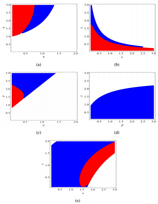
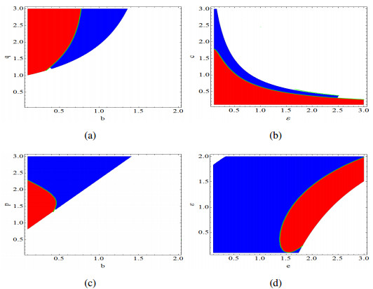
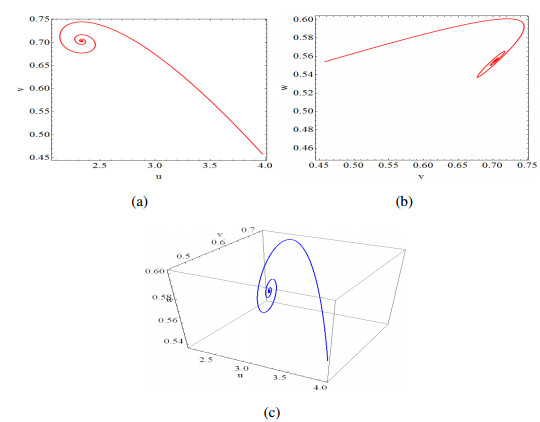
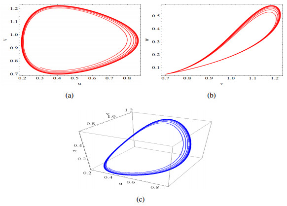
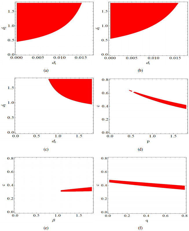
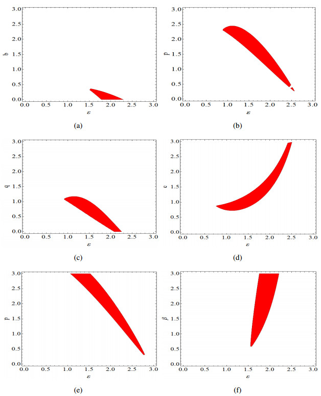
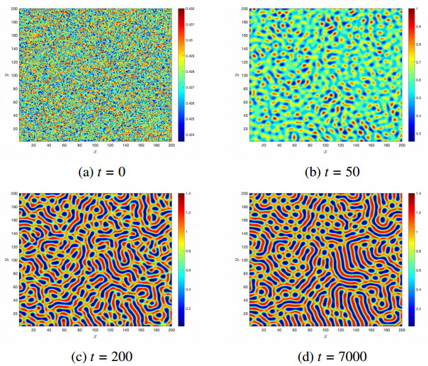
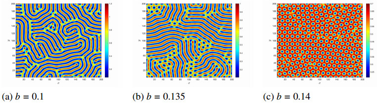
This paper formulates and analyzes a modified Previte-Hoffman food web with mixed functional responses. We investigate the existence, uniqueness, positivity and boundedness of the proposed model's solutions. The asymptotic local and global stability of the steady states are discussed. Analytical study of the proposed model reveals that it can undergo supercritical Hopf bifurcation. Furthermore, analysis of Turing instability in spatiotemporal version of the model is carried out where regions of pattern creation in parameters space are obtained. Using detailed numerical simulations for the diffusive and non-diffusive cases, the theoretical findings are verified for distinct sets of parameters.
Citation: A. Aldurayhim, A. Elsonbaty, A. A. Elsadany. Dynamics of diffusive modified Previte-Hoffman food web model[J]. Mathematical Biosciences and Engineering, 2020, 17(4): 4225-4256. doi: 10.3934/mbe.2020234
This paper formulates and analyzes a modified Previte-Hoffman food web with mixed functional responses. We investigate the existence, uniqueness, positivity and boundedness of the proposed model's solutions. The asymptotic local and global stability of the steady states are discussed. Analytical study of the proposed model reveals that it can undergo supercritical Hopf bifurcation. Furthermore, analysis of Turing instability in spatiotemporal version of the model is carried out where regions of pattern creation in parameters space are obtained. Using detailed numerical simulations for the diffusive and non-diffusive cases, the theoretical findings are verified for distinct sets of parameters.

| [1] |
R. T. Paine, Food web complexity and species diversity, Am. Nat., 100 (1966), 65-75. doi: 10.1086/282400

|
| [2] |
K. Fujii, Complexity-stability relationship of two-prey-one-predator species system model: Local and global stability, J. Theor. Biol., 69 (1977), 613-623. doi: 10.1016/0022-5193(77)90370-8
|
| [3] | J. D. Parrish, S. B. Saila, Interspecific competition, predation and species diversity, J. Theor. Biol., 27 (1970), 207-220. |
| [4] |
R. R. Vance, Predation and resource partitioning in one predator-two prey model communities, Am. Nat., 112 (1978), 797-813. doi: 10.1086/283324
|
| [5] | Y. Takeuchi, N. Adachi, Existence and bifurcation of stable equilibrium in two-prey, onepredator communities, Bull. Math. Biol., 45 (1983), 877-900. |
| [6] |
H. Kitano, Computational systems biology, Nature, 420 (2002), 206-210. doi: 10.1038/nature01254
|
| [7] |
J. A. Dunne, R. J. Williams, N. D. Martinez, Network structure and robustness of marine food webs, Mar. Ecol. Prog. Ser., 273 (2004), 291-302. doi: 10.3354/meps273291
|
| [8] | J. D. Murray, Mathematical biology, in Interdisciplinary Applied Mathematics, Springer, (2002). |
| [9] | L. D. Kuijper, B. W. Kooi, C. Zonneveld, S. A. Kooijman, Omnivory and food web dynamics, Ecol. Modell., 163 (2003), 19-32. |
| [10] | A. Al-Khedhairi, A. A. Elsadany, A. Elsonbaty, A. G. Abdelwahab, Dynamical study of a chaotic predator-prey model with an omnivore, Eur. Phys. J. Plus, 133 (2018), 29. |
| [11] |
A. M. Turing, The chemical basis of morphogenesis, Bull. Math. Biol., 52 (1990), 153-197. doi: 10.1016/S0092-8240(05)80008-4
|
| [12] | M. A. Chaplain, G. D. Singh, J. C. McLachlan, On growth and form: spatio-temporal pattern formation in biology, Wiley, (1999). |
| [13] | S. V. Petrovskii, H. Malchow, A minimal model of pattern formation in a prey-predator system, Math. Comput. Modell., 29 (1999), 49-63. |
| [14] |
H. Malchow, B. Radtke, M. Kallache, A. B. Medvinsky, D. A. Tikhonov, S. V. Petrovskii, Spatio-temporal pattern formation in coupled models of plankton dynamics and fish school motion, Nonlinear Anal. Real World Appl., 1 (2000), 53-67. doi: 10.1016/S0362-546X(99)00393-4
|
| [15] |
E. J. Crampin, W. W. Hackborn, P. K. Maini, Pattern formation in reaction-diffusion models with nonuniform domain growth, Bull. Math. Biol., 64 (2002), 747-769. doi: 10.1006/bulm.2002.0295
|
| [16] |
K. M. Page, P. K. Maini, N. A. Monk, Complex pattern formation in reaction-diffusion systems with spatially varying parameters, Phys. D Nonlinear Phenomena, 202 (2005), 95-115. doi: 10.1016/j.physd.2005.01.022
|
| [17] |
V. K. Vanag, I. R. Epstein, Design and control of patterns in reaction-diffusion systems, Chaos Interdiscip. J. Nonlinear Sci., 18 (2008), 026107. doi: 10.1063/1.2900555
|
| [18] | J. Murray, Mathematical Biology II: Spatial Models and Biomedical Applications, in Interdisciplinary Applied Mathematics, Springer, (2011). |
| [19] |
G. Gambino, M. C. Lombardo, M. Sammartino, Turing instability and pattern formation for the Lengyel-Epstein system with nonlinear diffusion, Acta Appl. Math., 132 (2014), 283-294. doi: 10.1007/s10440-014-9903-2
|
| [20] | L. Meng, Y. Han, Z. Lu, G. Zhang, Bifurcation, chaos, and pattern formation for the discrete predator-prey reaction-diffusion model, Discrete Dyn. Nat. Soc., 2019 (2019). |
| [21] |
J. A. Sherratt, Unstable wavetrains and chaotic wakes in reaction-diffusion systems of λ - ω type, Phys. D Nonlinear Phenomena, 82 (1995), 165-179. doi: 10.1016/0167-2789(94)00224-E
|
| [22] |
M. R. Owen, J. A. Sherratt, Pattern formation and spatiotemporal irregularity in a model for macrophage-tumour interactions, J. Theor. Biol., 189 (1997), 63-80. doi: 10.1006/jtbi.1997.0494
|
| [23] |
M. Pascual, M. Roy, A. Franc, A. Simple temporal models for ecological systems with complex spatial patterns, Ecol. Lett., 5 (2002), 412-419. doi: 10.1046/j.1461-0248.2002.00334.x
|
| [24] | L. A. D. Rodrigues, D. C. Mistro, S. Petrovskii, Pattern formation, long-term transients, and the Turing-Hopf bifurcation in a space-and time-discrete predator-prey system, Bull. Math. Biol., 73 (2011), 1812-1840. |
| [25] | K. Manna, M. Banerjee, Stationary, non-stationary and invasive patterns for a prey-predator system with additive Allee effect in prey growth, Ecol. Complexity, 36 (2018), 206-217. |
| [26] | K. Manna, V. Volpert, M. Banerjee, Dynamics of a Diffusive Two-Prey-One-Predator Model with Nonlocal Intra-Specific Competition for Both the Prey Species, Mathematics, 8 (2020), 101. |
| [27] | S. Petrovskii, K. Kawasaki, F. Takasu, N. Shigesada, Diffusive waves, dynamical stabilization and spatio-temporal chaos in a community of three competitive species, Jpn. J. Ind. Appl. Math.s, 18 (2001), 459. |
| [28] |
F. Rao, Spatiotemporal complexity of a three-species ratio-dependent food chain model, Nonlinear Dyn., 76 (2014), 1661-1676. doi: 10.1007/s11071-014-1237-0
|
| [29] | W. Abid, R. Yafia, M. A. Aziz-Alaoui, H. Bouhafa, A. Abichou, Diffusion driven instability and Hopf bifurcation in spatial predator-prey model on a circular domain, Appl. Math. Comput., 260 (2015), 292-313. |
| [30] |
Z. Xie, Cross-diffusion induced Turing instability for a three species food chain model, J. Math. Anal. Appl., 388 (2012), 539-547. doi: 10.1016/j.jmaa.2011.10.054
|
| [31] |
C. V. Pao, Dynamics of food-chain models with density-dependent diffusion and ratiodependent reaction function, J. Math. Anal. Appl., 433 (2016), 355-374. doi: 10.1016/j.jmaa.2015.05.075
|
| [32] |
Z. P. Ma, Y. X. Wang, Bifurcation of positive solutions for a three-species food chain model with diffusion, Comput. Math. Appl., 74 (2017), 3271-3282. doi: 10.1016/j.camwa.2017.08.015
|
| [33] |
N. Mukherjee, S. Ghorai, M. Banerjee, Detection of turing patterns in a three species food chain model via amplitude equation, Commun. Nonlinear Sci. Numer. Simul., 69 (2019), 219-236. doi: 10.1016/j.cnsns.2018.09.023
|
| [34] | N. Kumari, N. Mohan, Cross Diffusion Induced Turing Patterns in a Tritrophic Food Chain Model with Crowley-Martin Functional Response, Mathematics, 7 (2019), 229. |
| [35] | V. Weide Rodrigues, D. Cristina Mistro, L. A. Díaz Rodrigues, Pattern Formation and Bistability in a Generalist Predator-Prey Model, Mathematics, 8 (2020), 20. |
| [36] |
J. P. Previte, K. A. Hoffman, Period doubling cascades in a predator-prey model with a scavenger, Siam Rev., 55 (2013), 523-546. doi: 10.1137/110825911
|
| [37] | T. L. DeVault, O. E. Rhodes, J. A. Shivik, Scavenging by vertebrates: Behavioral, ecological, and evolutionary perspectives on an important energy transfer pathway in terrestrial ecosystems, Oikos, 102 (2003), 225-234. |
| [38] |
M. Kuznetsov, A. Kolobov, A. Polezhaev, Pattern formation in a reaction-diffusion system of Fitzhugh-Nagumo type before the onset of subcritical Turing bifurcation, Phys. Rev. E, 95 (2017), 052208. doi: 10.1103/PhysRevE.95.052208
|
| [39] | F. Bubba, C. Pouchol, N. Ferrand, G. Vidal, L. Almeida, B. Perthame, et al., A chemotaxisbased explanation of spheroid formation in 3D cultures of breast cancer cells, J. Theoretical Biol., 479 (2019), 73-80. |
| [40] |
L. N. Guin, B. Mondal, S. Chakravarty, Spatiotemporal Patterns of a Pursuit-evasion Generalist Predator-prey Model With Prey Harvesting, J. Appl. Nonlinear Dyn., 7 (2018), 165-177. doi: 10.5890/JAND.2018.06.005
|
| [41] |
D. Lacitignola, B. Bozzini, M. Frittelli, I. Sgura, Turing pattern formation on the sphere for a morphochemical reaction-diffusion model for electrodeposition, Commun. Nonlinear Sci. Numer. Simul., 48 (2017), 484-508. doi: 10.1016/j.cnsns.2017.01.008
|
| [42] |
W. Abid, R. Yafia, M. A. Aziz-Alaoui, A. Aghriche, Turing Instability and Hopf Bifurcation in a Modified Leslie-Gower Predator-Prey Model with Cross-Diffusion, Int. J. Bifurcation Chaos, 28 (2018), 1850089. doi: 10.1142/S021812741850089X
|
| [43] | M. Bär, Reaction-diffusion patterns and waves: From chemical reactions to cardiac arrhythmias, in Spirals and Vortices, Springer, (2019). |
| [44] |
M. Baurmann, T. Gross, U. Feudel, Instabilities in spatially extended predator-prey systems: Spatio-temporal patterns in the neighborhood of Turing-Hopf bifurcations, J. Theoretical Biol., 245 (2007), 220-229. doi: 10.1016/j.jtbi.2006.09.036
|
| [45] | S. H. Strogatz, Nonlinear dynamics and chaos with student solutions manual: With applications to physics, biology, chemistry, and engineering, CRC press, (2018). |
Figures(14)

A. Aldurayhim, A. Elsonbaty, A. A. Elsadany. Dynamics of diffusive modified Previte-Hoffman food web model[J]. Mathematical Biosciences and Engineering, 2020, 17(4): 4225-4256. doi: 10.3934/mbe.2020234


 DownLoad: