Fear effect in a three-species food chain model with generalist predator

Soumitra Pal; Pankaj Kumar Tiwari; Arvind Kumar Misra; Hao Wang; Soumitra Pal; Pankaj Kumar Tiwari; Arvind Kumar Misra; Hao Wang

doi:10.3934/mbe.2024001

Mathematical Biosciences and Engineering

2024, Volume 21, Issue 1: 1-33. doi: 10.3934/mbe.2024001

Previous Article Next Article

Research article

Fear effect in a three-species food chain model with generalist predator

1.
Department of Mathematics, Institute of Science, Banaras Hindu University, Varanasi 221005, India
2.
Department of Basic Science and Humanities, Indian Institute of Information Technology, Bhagalpur 813210, India
3.
Department of Mathematical and Statistical Science, University of Alberta, Edmonton AB T6G 2G1, Canada

Received: 18 October 2023 Revised: 19 November 2023 Accepted: 27 November 2023 Published: 08 December 2023

Within the framework of a food web, the foraging behavior of meso-carnivorous species is influenced by fear responses elicited by higher trophic level species, consequently diminishing the fecundity of these species. In this study, we investigate a three-species food chain model comprising of prey, an intermediate predator, and a top predator. We assume that both the birth rate and intraspecies competition of prey are impacted by fear induced by the intermediate predator. Additionally, the foraging behavior of the intermediate predator is constrained due to the presence of the top predator. It is essential to note that the top predators exhibit a generalist feeding behavior, encompassing food sources beyond the intermediate predators. The study systematically determines all feasible equilibria of the proposed model and conducts a comprehensive stability analysis of these equilibria. The investigation reveals that the system undergoes Hopf bifurcation concerning various model parameters. Notably, when other food sources significantly contribute to the growth of the top predators, the system exhibits stable behavior around the interior equilibrium. Our findings indicate that the dynamic influence of fear plays a robust role in stabilizing the system. Furthermore, a cascading effect within the system, stemming from the fear instigated by top predators, is observed and analyzed. Overall, this research sheds light on the intricate dynamics of fear-induced responses in shaping the stability and behavior of multi-species food web systems, highlighting the profound cascading effects triggered by fear mechanisms in the ecosystem.
- food chain model,
- generalist predator,
- fear effect, Hopf bifurcation,
- stability region
Citation: Soumitra Pal, Pankaj Kumar Tiwari, Arvind Kumar Misra, Hao Wang. Fear effect in a three-species food chain model with generalist predator[J]. Mathematical Biosciences and Engineering, 2024, 21(1): 1-33. doi: 10.3934/mbe.2024001

Related Papers:

Abstract

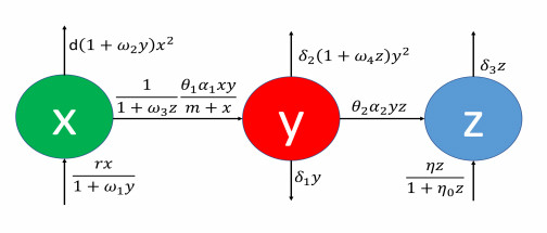
Within the framework of a food web, the foraging behavior of meso-carnivorous species is influenced by fear responses elicited by higher trophic level species, consequently diminishing the fecundity of these species. In this study, we investigate a three-species food chain model comprising of prey, an intermediate predator, and a top predator. We assume that both the birth rate and intraspecies competition of prey are impacted by fear induced by the intermediate predator. Additionally, the foraging behavior of the intermediate predator is constrained due to the presence of the top predator. It is essential to note that the top predators exhibit a generalist feeding behavior, encompassing food sources beyond the intermediate predators. The study systematically determines all feasible equilibria of the proposed model and conducts a comprehensive stability analysis of these equilibria. The investigation reveals that the system undergoes Hopf bifurcation concerning various model parameters. Notably, when other food sources significantly contribute to the growth of the top predators, the system exhibits stable behavior around the interior equilibrium. Our findings indicate that the dynamic influence of fear plays a robust role in stabilizing the system. Furthermore, a cascading effect within the system, stemming from the fear instigated by top predators, is observed and analyzed. Overall, this research sheds light on the intricate dynamics of fear-induced responses in shaping the stability and behavior of multi-species food web systems, highlighting the profound cascading effects triggered by fear mechanisms in the ecosystem.

References

[1]	A. J. Lotka, Elements of Physical Biology, Williams and Wilkins Company, Baltimore, 1925.
[2]	V. Volterra, Variations and fluctuations of the number of individuals in animal species living together, Anim. Ecol., (1926), 409–448.
[3]	P. Cong, M. Fan, X. Zou, Dynamic of three-species food chain model with fear effect, Commun. Nonlinear Sci. Numer. Simul., 99 (2021), 105809. https://doi.org/10.1016/j.cnsns.2021.105809 doi: 10.1016/j.cnsns.2021.105809
[4]	A. Erbach, F. Lutscher, G. Seo, Bistability and limit cycles in generalist predator-prey dynamics, Ecol. Complex., 14 (2013), 48–55. https://doi.org/10.1016/j.ecocom.2013.02.005 doi: 10.1016/j.ecocom.2013.02.005
[5]	C. Magal, C. G. Cosner, S. Ruan, J. Casas, Control of invasive hosts by generalist parasitoids Math. Med. Biol., 25 (2008), 1–20. https://doi.org/10.1093/imammb/dqm011 doi: 10.1093/imammb/dqm011
[6]	M. Verma, A. K. Misra, Modeling the effect of prey refuge on a ratio-dependent predator–prey system with the Allee effect, Bull. Math. Biol., 80 (2018), 626–656. https://doi.org/10.1007/s11538-018-0394-6 doi: 10.1007/s11538-018-0394-6
[7]	X. Wang, L. Zanette, X. Zou, Modelling the fear effect in predator-prey interactions, J. Math. Biol., 73 (2016), 1179–1204. https://doi.org/10.1007/s00285-016-0989-1 doi: 10.1007/s00285-016-0989-1
[8]	Y. Xu, A. L. Krause, R. A. Van Gorder, Generalist predator dynamics under kolmogorov versus non-Kolmogorov models, J. Theor. Biol., 486 (2020), 110060. https://doi.org/10.1016/j.jtbi.2019.110060 doi: 10.1016/j.jtbi.2019.110060
[9]	M. W. Sabelis, Predatory arthropods, in Natural Enemies: the Population Biology of Predators, Parasites and Diseases, (1992), 225–264.
[10]	M. G. Solomon, J. V. Cross, J. D. Fitzgerald, C. A. M. Campbell, R. L. Jolly, R. W. Olszak, et al., Biocontrol of pests of apples and pears in northern and central Europe-3. Predators, Biocontrol Sci. Technol., 10 (2000), 91–128. https://doi.org/10.1080/09583150029260 doi: 10.1080/09583150029260
[11]	H. Triltsch, Gut contents in field sampled adults of Coccinella septem-punctata (Col.: Coccinellidae), BioControl, 42 (1997), 125–131. https://doi.org/10.1007/BF02769889 doi: 10.1007/BF02769889
[12]	J. P. Harmon, A. R. Ives, J. E. Losey, A. C. Olson, K. S. Rauwald, Colemegilla maculata (Coleoptera: Coccinellidae) predation on pea aphids promoted by proximity to dandelions, Oecologia, 125 (2000), 543–548. https://doi.org/10.1007/s004420000476 doi: 10.1007/s004420000476
[13]	C. Roger, D. Coderre, G. Boivin, Differential prey utilization by the generalist predator Coleomegilla maculata lengi according to prey size and species, Entomol. Exp. Appl., 94 (2000), 3–13. https://doi.org/10.1046/j.1570-7458.2000.00598.x doi: 10.1046/j.1570-7458.2000.00598.x
[14]	B. Mondal, S. Sarkar, U. Ghosh, Complex dynamics of a generalist predator-prey model with hunting cooperation in predator, Eur. Phys. J. Plus, 137 (2022). https://doi.org/10.1140/epjp/s13360-021-02272-4 doi: 10.1140/epjp/s13360-021-02272-4
[15]	S. Creel, D. Christianson, Relationships between direct predation and risk effects, Trends Ecol. Evol., 23 (2008), 194–201. https://doi.org/10.1016/j.tree.2007.12.004 doi: 10.1016/j.tree.2007.12.004
[16]	B. L. Peckarsky, P. A. Abrams, D. I. Bolnick, L. M. Dill, J. H. Grabowski, B. Luttbeg, et al., Revisiting the classics: considering nonconsumptive effects in textbook examples of predator-prey interactions, Ecology, 89 (2008), 2416–2425.
[17]	J. Winnie, S. Creel, The many effects of carnivores on their prey and their implications for trophic cascades, and ecosystem structure and function, Food Webs, 12 (2017), 88–94. https://doi.org/10.1016/j.fooweb.2016.09.002 doi: 10.1016/j.fooweb.2016.09.002
[18]	L. Y. Zanette, A. F. White, M. C. Allen, M. Clinchy, Perceived predation risk reduces the number of offspring songbirds produce per year, Science, 334 (2011), 1398–1401. https://doi.org/10.1126/science.1210908 doi: 10.1126/science.1210908
[19]	M. J. Sheriff, C. J. Krebs, R. Boonstra, The sensitive hare: sublethal effects of predator stress on reproduction in snowshoe hares, J. Anim. Ecol., 78 (2009), 1249–1258. https://doi.org/10.1111/j.1365-2656.2009.01552.x doi: 10.1111/j.1365-2656.2009.01552.x
[20]	J. P. Suraci, M. Clinchy, L. M. Dill, D. Roberts, L. Y. Zanette, Fear of large carnivores causes a trophic cascade, Nat. Commun., 7 (2016), 10698. https://doi.org/10.1038/ncomms10698 doi: 10.1038/ncomms10698
[21]	W. Cresswell, Predation in bird populations, J. Ornithol., 152 (2011), 251–263.
[22]	E. L. Preisser, D. I. Bolnick, The many faces of fear: comparing the pathways and impacts of non-consumptive predator effects on prey populations, PLoS One, 3 (2008), e2465. https://doi.org/10.1371/journal.pone.0002465 doi: 10.1371/journal.pone.0002465
[23]	K. B. Altendrof, J. W. Laundre, C. A. Lopez Gonzalez, J. S. Brown, Assessing effects of predation risk on foraging behaviour of mule deer, J. Mammal., 82 (2001), 430–439. https://doi.org/10.1644/1545-1542(2001)082<0430:AEOPRO>2.0.CO;2 doi: 10.1644/1545-1542(2001)082<0430:AEOPRO>2.0.CO;2
[24]	S. Creel, D. Christianson, S. Liley, J. A. Winnie, Predation risk affects reproductive physiology and demography of elk, Science, 315 (2007), 960. https://doi.org/10.1126/science.1135918 doi: 10.1126/science.1135918
[25]	S. Creel, J. Winnie Jr, B. Maxwell, K. Hamlin, M. Creel, Elk alter habitat selection as an antipredator response to wolves, Ecology, 86 (2005), 3387–3397. https://doi.org/10.1890/05-0032 doi: 10.1890/05-0032
[26]	F. Hua, K. E. Sieving, R. J. Fletcher Jr, C. A. Wright, Increased perception of predation risk to adults and offspring alters avian reproductive strategy and performance, Behav. Ecol., 25 (2014), 509–519. https://doi.org/10.1093/beheco/aru017 doi: 10.1093/beheco/aru017
[27]	S. Pal, N. Pal, S. Samanta, J. Chattopadhyay, Fear effect in prey and hunting cooperation among predators in a Leslie–Gower model, Math. Biosci. Eng., 16 (2019), 5146–5179. https://doi.org/10.3934/mbe.2019258 doi: 10.3934/mbe.2019258
[28]	S. Pal, A. Gupta, A. K. Misra, B. Dubey, Chaotic dynamics of a stage–structured prey–predator system with hunting cooperation and fear in presence of two discrete delays, J. Biol. Syst., 31 (2023), 611–642. https://doi.org/10.1142/S0218339023500213 doi: 10.1142/S0218339023500213
[29]	S. Pal, P. Panday, N. Pal, A. K. Misra, J. Chattopadhyay, Dynamical behaviors of a constant prey refuge ratio–dependent prey–predator model with Allee and fear effects, Int. J. Biomath., 17 (2023), 2350010. https://doi.org/10.1142/S1793524523500109 doi: 10.1142/S1793524523500109
[30]	S. K. Sasmal, Population dynamics with multiple Allee effects induced by fear factors: a mathematical study on prey-predator interactions, Appl. Math. Model., 64 (2018), 1–14. https://doi.org/10.1016/j.apm.2018.07.021 doi: 10.1016/j.apm.2018.07.021
[31]	P. K. Tiwari, M. Verma, S. Pal, Y. Kang, A. K. Misra, A delay nonautonomous predator–prey model for the effects of fear, refuge and hunting cooperation, J. Biol. Syst., 29 (2020), 927–969. https://doi.org/10.1142/S0218339021500236 doi: 10.1142/S0218339021500236
[32]	R. K. Upadhyay, S. Mishra, Population dynamic consequences of fearful prey in a spatiotemporal predator–prey system, Math. Biosci. Eng., 16 (2018), 338–372. https://doi.org/10.3934/mbe.2019017 doi: 10.3934/mbe.2019017
[33]	J. Wang, Y. Cai, S. Fu, W. Wang, The effect of the fear factor on the dynamics of a predator–prey model incorporating the prey refuge, Chaos, 29 (2019), 083109. https://doi.org/10.1063/1.5111121 doi: 10.1063/1.5111121
[34]	H. Zhang, Y. Cai, S. Fu, W. Wang, Impact of the fear effect in a prey–predator model incorporating a prey refuge, Appl. Math. Comput., 356 (2019), 328–337. https://doi.org/10.1016/j.amc.2019.03.034 doi: 10.1016/j.amc.2019.03.034
[35]	D. Mukherjee, Role of fear in predator-prey system with intraspecific competition, Math. Comput. Simul., 177 (2020), 263–275. https://doi.org/10.1016/j.matcom.2020.04.025 doi: 10.1016/j.matcom.2020.04.025
[36]	B. Mondal, S. Roy, U. Ghosh, P. K. Tiwari, A systematic study of autonomous and nonautonomous predator-prey models for the combined effects of fear, refuge, cooperation and harvesting, Eur. Phys. J. Plus, 137 (2022). https://doi.org/10.1140/epjp/s13360-022-02915-0 doi: 10.1140/epjp/s13360-022-02915-0
[37]	P. Panday, N. Pal, S. Samanta, J. Chattopadhyay, A three species food chain model with fear induced trophic cascade, Int. J. Appl. Comput. Math., 5 (2019), 1–26. https://doi.org/10.1007/s40819-019-0688-x doi: 10.1007/s40819-019-0688-x
[38]	M. C. Allen, M. Clinchy, L. Y. Zanette, Fear of predators in free–living wildlife reduces population growth over generations, PNAS, 119 (2022), e2112404119. https://doi.org/10.1073/pnas.211240411 doi: 10.1073/pnas.211240411
[39]	M. Clinchy, M. J. Sheriff, L. Y. Zanette, Predator-induced stress and the ecology of fear, Funct. Ecol., 27 (2013), 56–65. https://doi.org/10.1111/1365-2435.12007 doi: 10.1111/1365-2435.12007
[40]	M. J. Sheriff, S. D. Peacor, D. Hawlena, M. Thaker, Non–consumptive predator effects on prey population size: A dearth of evidence, J. Anim. Ecol., 89 (2020), 1302–1316. https://doi.org/10.1111/1365-2656.13213 doi: 10.1111/1365-2656.13213
[41]	C. E. Gordon, A. Feit, J. Gruber, M. Lentic, Mesopredator suppression by an apex predator alleviates the risk of predation perceived by small prey, Proc. R. Soc. B, 282 (2015), 20142870. https://doi.org/10.1098/rspb.2014.2870 doi: 10.1098/rspb.2014.2870
[42]	W. J. Ripple, R. L. Beschta, Trophic cascades in Yellowstone: The first 15 years after wolf reintroduction, Biol. Conserv., 145 (2012), 205–213. https://doi.org/10.1016/j.biocon.2011.11.005 doi: 10.1016/j.biocon.2011.11.005
[43]	J. K. Hale, Theory of Functional Differential Equations, Springer, New York, 1977.
[44]	L. Perko, Differential Equation and Dynamical System, Springer, New York, 2001.
[45]	P. Liu, J. Shi, Y. Wang, Bifurcation from a degenerate simple eigenvalue, J. Funct. Anal., 264 (2013), 2269–2299. https://doi.org/10.1016/j.jfa.2013.02.010 doi: 10.1016/j.jfa.2013.02.010
[46]	B. Hassard, N. Kazarinoff, Y. Wan, Theory and Applications of Hopf Bifurcation, CUP Archive Cmbridge, 1981.
[47]	S. M. Blower, M. Dowlatabadi, Sensitivity and uncertainty analysis of complex models of disease transmission: an HIV model, as an example, Int. Stat. Rev., 62 (1994), 229–243. https://doi.org/10.2307/1403510 doi: 10.2307/1403510
[48]	S. Marino, I. B. Hogue, C. J. Ray, D. E. Kirschner, A methodology for performing global uncertainty and sensitivity analysis in systems biology, J. Theor. Biol., 254 (2008), 178–196. https://doi.org/10.1016/j.jtbi.2008.04.011 doi: 10.1016/j.jtbi.2008.04.011
[49]	P. Panday, N. Pal, S. Samanta, P. Tryjanowski, J. Chattopadhyay, Dynamics of a stage–structured predator–prey model: cost and benefit of fear–induced group defense, J. Theor. Biol., 528 (2021), 110846. https://doi.org/10.1016/j.jtbi.2021.110846 doi: 10.1016/j.jtbi.2021.110846

Reader Comments

Your name:*

Email:*
© 2024 the Author(s), licensee AIMS Press. This is an open access article distributed under the terms of the Creative Commons Attribution License (http://creativecommons.org/licenses/by/4.0)