Finite-time synchronization of fractional-order heterogeneous dynamical networks with impulsive interference via aperiodical intermittent control

Tao Xie; Xing Xiong; Tao Xie; Xing Xiong

doi:10.3934/math.2025287

AIMS Mathematics

2025, Volume 10, Issue 3: 6291-6317. doi: 10.3934/math.2025287

Previous Article Next Article

Research article

Finite-time synchronization of fractional-order heterogeneous dynamical networks with impulsive interference via aperiodical intermittent control

Tao Xie ^,,
Xing Xiong

School of Mathematics and Statistics, Hubei Normal University, Huangshi, 435002, China

Received: 10 December 2024 Revised: 18 February 2025 Accepted: 27 February 2025 Published: 20 March 2025
MSC : 93B35, 93D23

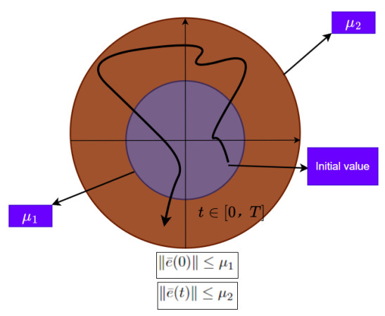
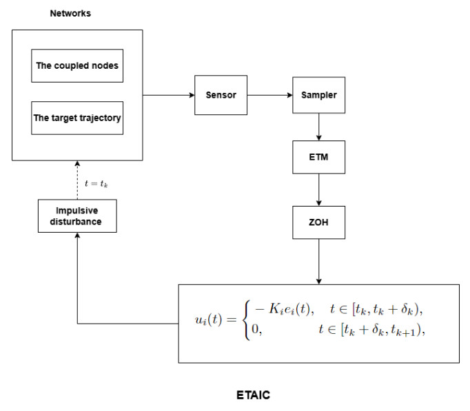
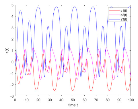
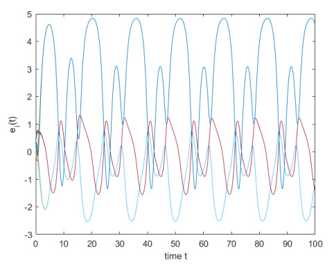
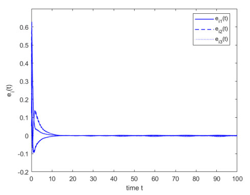
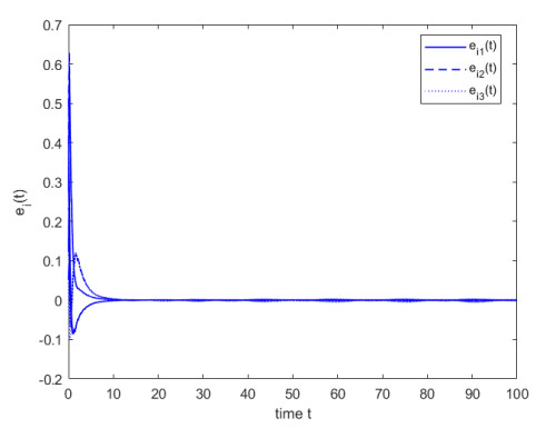
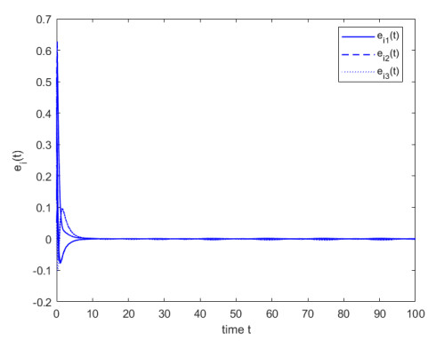
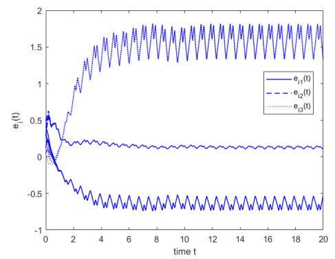
This paper addresses the problem of ensuring finite-time synchronization for fractional-order heterogeneous dynamical networks via aperiodic intermittent control, where uncertain impulsive disturbances are introduced at the instants triggered by the control actions applied to the system. Under aperiodic time-triggered and event-triggered intermittent control, a Lyapunov function iteration method, based on the traditional Lyapunov method, was developed to analyze the criteria for finite-time synchronization. Several sufficient conditions were proposed to ensure finite-time synchronization. First, within the framework of finite-time and time-triggered control, the relationship between the control period width, impulsive disturbances, and configuration control parameters was established to guarantee finite-time synchronization. Second, an event-triggered mechanism was introduced into the intermittent control, where the sequence of impulsive disturbance instants was determined by a pre-designed trigger threshold. The relationship between impulsive disturbances, the event-triggered threshold, and the control period width was established. These two relationships can potentially increase the flexibility of the designed control periods and control width. Moreover, the Zeno phenomenon can be eliminated in the event-triggered mechanism. Finally, two simulations were presented to illustrate the feasibility and effectiveness of the theoretical results.
- fractional-order heterogeneous dynamical networks,
- impulsive,
- finite-time synchronization,
- aperiodic intermittent control,
- event-triggered mechanism
Citation: Tao Xie, Xing Xiong. Finite-time synchronization of fractional-order heterogeneous dynamical networks with impulsive interference via aperiodical intermittent control[J]. AIMS Mathematics, 2025, 10(3): 6291-6317. doi: 10.3934/math.2025287

Related Papers:

Abstract

This paper addresses the problem of ensuring finite-time synchronization for fractional-order heterogeneous dynamical networks via aperiodic intermittent control, where uncertain impulsive disturbances are introduced at the instants triggered by the control actions applied to the system. Under aperiodic time-triggered and event-triggered intermittent control, a Lyapunov function iteration method, based on the traditional Lyapunov method, was developed to analyze the criteria for finite-time synchronization. Several sufficient conditions were proposed to ensure finite-time synchronization. First, within the framework of finite-time and time-triggered control, the relationship between the control period width, impulsive disturbances, and configuration control parameters was established to guarantee finite-time synchronization. Second, an event-triggered mechanism was introduced into the intermittent control, where the sequence of impulsive disturbance instants was determined by a pre-designed trigger threshold. The relationship between impulsive disturbances, the event-triggered threshold, and the control period width was established. These two relationships can potentially increase the flexibility of the designed control periods and control width. Moreover, the Zeno phenomenon can be eliminated in the event-triggered mechanism. Finally, two simulations were presented to illustrate the feasibility and effectiveness of the theoretical results.

References

[1]	A. L. Barabâsi, H. Jeong, Z. Néda, E. Ravasz, A. Schubert, T. Vicsek, Evolution of the social network of scientific collaborations, Physica A, 311 (2002), 590–614.
[2]	S. Nara, P. Davis, H. Totsuji, Memory search using complex dynamics in a recurrent neural network model, Neural Networks, 311 (1993), 963–973. https://doi.org/10.1016/S0893-6080(09)80006-3 doi: 10.1016/S0893-6080(09)80006-3
[3]	R. Pastor-Satorras, E. Smith, R. V. Solé, Evolving protein interaction networks through gene duplication, J. Theor. Biol., 222 (2003), 199–210. https://doi.org/10.1016/S0022-5193(03)00028-6 doi: 10.1016/S0022-5193(03)00028-6
[4]	A. A. Kilbas, H. M. Srivastava, J. J. Trujillo, Theory and applications of fractional differential equations, Elsevier, 2006,204.
[5]	E. Reyes-Melo, J. Martinez-Vega, C. Guerrero-Salazar, U. Ortiz-Mendez, Application of fractional calculus to the modeling of dielectric relaxation phenomena in polymeric materials, J. Appl. Polym. Sci., 98 (2005), 923–935. https://doi.org/10.1002/app.22057 doi: 10.1002/app.22057
[6]	Z. Ding, H. Zhang, Z. Zeng, L. Yang, S. Li, Global dissipativity and quasi mittag leffler synchronization of fractional-order discontinuous complex-valued neural networks, IEEE T. Neur. Net. Lear., 34 (2021), 4139–4152. https://doi.org/10.1109/TNNLS.2021.3119647 doi: 10.1109/TNNLS.2021.3119647
[7]	S. Zhang, Y. Yu, H. Wang, Mittag-leffler stability of fractional-order hopfield neural networks, Nonlinear Anal.-Hybri., 16 (2015), 104–121. https://doi.org/10.1016/j.nahs.2014.10.001 doi: 10.1016/j.nahs.2014.10.001
[8]	L. Xu, W. Liu, H. Hu, W. Zhou, Exponential ultimate boundedness of fractional-order differential systems via periodically intermittent control, Nonlinear Dynam., 96 (2019), 1665–1675. https://doi.org/10.1007/s11071-019-04877-y doi: 10.1007/s11071-019-04877-y
[9]	W. M. Haddad, V. Chellaboina, S. G. Nersesov, Impulsive and hybrid dynamical systems: Stability, dissipativity, and control, Princeton University Press, 2006.
[10]	Q. Song, H. Yan, Z. Zhao, Y. Liu, Global exponential stability of complex-valued neural networks with both time-varying delays and impulsive effects, Neural Networks, 79 (2016), 108–116. https://doi.org/10.1016/j.neunet.2016.03.007 doi: 10.1016/j.neunet.2016.03.007
[11]	Q. Cui, L. Li, L. Wang, Exponential stability of delayed nonlinear systems with state-dependent delayed impulses and its application in delayed neural networks, Commun. Nonlinear Sci., 215 (2023), 107375. https://doi.org/10.1016/j.cnsns.2023.107375 doi: 10.1016/j.cnsns.2023.107375
[12]	J. Suo, J. Sun, Asymptotic stability of differential systems with impulsive effects suffered by logic choice, Automatica, 51 (2015), 302–307. https://doi.org/10.1016/j.automatica.2014.10.090 doi: 10.1016/j.automatica.2014.10.090
[13]	Z. Shen, C. Li, H. Li, Z. Cao, Estimation of the domain of attraction for discrete-time linear impulsive control systems with input saturation, Appl. Math. Comput., 362 (2019), 124502. https://doi.org/10.1016/j.amc.2019.06.016 doi: 10.1016/j.amc.2019.06.016
[14]	X. Zhang, C. Li, H. Li, Finite-time stabilization of nonlinear systems via impulsive control with state-dependent delay, J. Franklin I., 359 (2022), 1196–1214. https://doi.org/10.1016/j.jfranklin.2021.11.013 doi: 10.1016/j.jfranklin.2021.11.013
[15]	J. Zhang, W. H. Chen, X. Lu, Robust fuzzy stabilization of nonlinear time-delay systems subject to impulsive perturbations, Commun. Nonlinear Sci., 80 (2020), 104953. https://doi.org/10.1016/j.cnsns.2019.104953 doi: 10.1016/j.cnsns.2019.104953
[16]	H. L. Li, J. Cao, H. Jiang, A. Alsaedi, Graph theory-based finite-time synchronization of fractional-order complex dynamical networks, J. Franklin I., 355 (2018), 5771–5789. https://doi.org/10.1016/j.jfranklin.2018.05.039 doi: 10.1016/j.jfranklin.2018.05.039
[17]	J. M. He, L. J. Pei, Function matrix projection synchronization for the multi-time delayed fractional order memristor-based neural networks with parameter uncertainty, Appl. Math. Comput., 454 (2023), 128110. https://doi.org/10.1016/j.amc.2023.128110 doi: 10.1016/j.amc.2023.128110
[18]	J. M. He, L. J. Pei, Function matrix projective synchronization for unknown and delayed fractional-order neural network, Neural Comput. Appl., 15 (2023), 17941–17952. https://doi.org/10.1007/s00521-023-08641-7 doi: 10.1007/s00521-023-08641-7
[19]	L. Xu, W. Liu, H. Hu, W. Zhou, Exponential ultimate boundedness of fractional-order differential systems via periodically intermittent control, Nonlinear Dynam., 96 (2019), 1665–1675. https://doi.org/10.1007/s11071-019-04877-y doi: 10.1007/s11071-019-04877-y
[20]	S. Cai, X. Li, P. Zhou, J. Shen, Aperiodic intermittent pinning control for exponential synchronization of memristive neural networks with time-varying delays, Neurocomputing, 332 (2019), 249–258. https://doi.org/10.1016/j.neucom.2018.12.070 doi: 10.1016/j.neucom.2018.12.070
[21]	F. Wang, Y. Yang, Intermittent synchronization of fractional order coupled nonlinear systems based on a new differential inequality, Physica A, 512 (2018), 142–152. https://doi.org/10.1016/j.physa.2018.08.023 doi: 10.1016/j.physa.2018.08.023
[22]	Y. Xu, S. Gao, W. Li, Exponential stability of fractional-order complex multi-links networks with aperiodically intermittent control, IEEE T. Neur. Net. Lear., 32 (2020), 4063–4074. https://doi.org/10.1109/TNNLS.2020.3016672 doi: 10.1109/TNNLS.2020.3016672
[23]	H. L. Li, C. Hu, H. Jiang, Z. Teng, Y. L. Jiang, Synchronization of fractional-order complex dynamical networks via periodically intermittent pinning control, Chaos Soliton. Fract., 103 (2017), 357–363. https://doi.org/10.1016/j.chaos.2017.06.025 doi: 10.1016/j.chaos.2017.06.025
[24]	S. Cai, M. Hou, Quasi-synchronization of fractional-order heterogeneous dynamical networks via aperiodic intermittent pinning control, Chaos Soliton. Fract., 146 (2021), 110901. https://doi.org/10.1016/j.chaos.2021.110901 doi: 10.1016/j.chaos.2021.110901
[25]	Y. Yang, Y. He, M. Wu, Intermittent control strategy for synchronization of fractional-order neural networks via piecewise lyapunov function method, J. Franklin I., 356 (2019), 4648–4676. https://doi.org/10.1016/j.jfranklin.2018.12.020 doi: 10.1016/j.jfranklin.2018.12.020
[26]	L. Zhang, J. Zhong, J. Lu, Intermittent control for finite-time synchronization of fractional-order complex networks, Neural Networks, 144 (2021), 11–20. https://doi.org/10.1016/j.neunet.2021.08.004 doi: 10.1016/j.neunet.2021.08.004
[27]	Y. Wang, C. Li, H. Wu, H. Deng, Stabilization of nonlinear delayed systems subject to impulsive disturbance via aperiodic intermittent control, J. Franklin I., 361 (2014), 106675. https://doi.org/10.1016/j.jfranklin.2024.106675 doi: 10.1016/j.jfranklin.2024.106675
[28]	L. You, X. Yang, S. Wu, X. Li, Finite-time stabilization for uncertain nonlinear systems with impulsive disturbance via aperiodic intermittent control, Appl. Math. Comput., 443 (2023), 127782. https://doi.org/10.1016/j.amc.2022.127782 doi: 10.1016/j.amc.2022.127782
[29]	Y. Zhou, H. Zhang, Z. Zeng, Synchronization of memristive neural networks with unknown parameters via event-triggered adaptive control, Neural Networks, 319 (2021), 255–264. https://doi.org/10.1016/j.neunet.2021.02.029 doi: 10.1016/j.neunet.2021.02.029
[30]	J. Bai, H. Wu, J. Cao, Topology identification for fractional complex networks with synchronization in finite time based on adaptive observers and event-triggered control, Neurocomputing, 505 (2022), 166–177. https://doi.org/10.1016/j.neucom.2022.07.023 doi: 10.1016/j.neucom.2022.07.023
[31]	Y. Tan, M. Xiong, B. Zhang, S. Fei, Adaptive event-triggered nonfragile state estimation for fractional-order complex networked systems with cyber attacks, IEEE T. Syst. Man. Cy.-A, 52 (2021), 2121–2133. https://doi.org/10.1109/TSMC.2021.3049231 doi: 10.1109/TSMC.2021.3049231
[32]	Z. Yu, S. Yu, H. Jiang, Finite/fixed-time event-triggered aperiodic intermittent control for nonlinear systems, Chaos Soliton. Fract., 173 (2023), 113735. https://doi.org/10.1016/j.chaos.2023.113735 doi: 10.1016/j.chaos.2023.113735
[33]	B. Liu, M. Yang, B. Xu, G. Zhang, Exponential stabilization of continuous-time dynamical systems via time and event triggered aperiodic intermittent control, Appl. Math. Comput., 398 (2021), 125713. https://doi.org/10.1016/j.amc.2020.125713 doi: 10.1016/j.amc.2020.125713
[34]	F. Lin, G. Xue, B. Qin, S. Li, H. Liu, Event-triggered finite-time fuzzy control approach for fractional-order nonlinear chaotic systems with input delay, Chaos Soliton. Fract., 175 (2023), 114036. https://doi.org/10.1016/j.chaos.2023.114036 doi: 10.1016/j.chaos.2023.114036
[35]	J. Zhuang, S. Peng, Y. Wang, Event-triggered intermittent-based impulsive control for stabilization of nonlinear systems, IEEE T. Circuits-Ii, 69 (2022), 5039–5043. https://doi.org/10.1109/TCSII.2022.3204570 doi: 10.1109/TCSII.2022.3204570
[36]	X. Yang, J. Lam, D. W. Ho, Z. Feng, Fixed-time synchronization of complex networks with impulsive effects via nonchattering control, IEEE T. Automat. Contr., 62 (2017), 5511–5521. https://doi.org/10.1109/TAC.2017.2691303 doi: 10.1109/TAC.2017.2691303
[37]	X. He, X. Li, S. Song, Finite-time input-to-state stability of nonlinear impulsive systems, Automatica, 135 (2022), 109994. https://doi.org/10.1016/j.automatica.2021.109994 doi: 10.1016/j.automatica.2021.109994
[38]	F. Du, J. G. Lu, Q. H. Zhang, Delay-dependent finite-time synchronization criterion of fractional-order delayed complex networks, Commun. Nonlinear Sci., 119 (2023), 107072. https://doi.org/10.1016/j.cnsns.2022.107072 doi: 10.1016/j.cnsns.2022.107072
[39]	H. L. Li, J. Cao, H. Jiang, A. Alsaedi, Graph theory-based finite-time synchronization of fractional-order complex dynamical networks, J. Franklin I., 355 (2018), 5771–5789. https://doi.org/10.1016/j.jfranklin.2018.05.039 doi: 10.1016/j.jfranklin.2018.05.039
[40]	Y. Li, Y. Kao, C. Wang, H. Xia, Fnite-time synchronization of delayed fractional-order heterogeneous complex networks, Neurocomputing, 384 (2020), 368–375. https://doi.org/10.1016/j.neucom.2019.11.043 doi: 10.1016/j.neucom.2019.11.043

Reader Comments

Your name:*

Email:*
© 2025 the Author(s), licensee AIMS Press. This is an open access article distributed under the terms of the Creative Commons Attribution License (http://creativecommons.org/licenses/by/4.0)