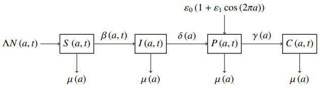
Immunotherapy is a targeted therapy that can be applied to cervical cancer patients to prevent DNA damage caused by human papillomavirus (HPV). The HPV infects normal cervical cells withing a specific cell age interval, i.e., between the $ G_1 $ to $ S $ phase of the cell cycle. In this study, we developed a new mathematical model of age-dependent immunotherapy for cervical cancer. The model is a four-dimensional first-order partial differential equation with time- and age-independent variables. The cell population is divided into four sub-populations, i.e., susceptible cells, cells infected by HPV, precancerous cells, and cancer cells. The immunotherapy term has been added to precancerous cells since these cells can experience regression if appointed by proper treatments. The immunotherapy process is closely related to the rate of T-cell division. The treatment works in the same cell cycle that stimulates and inhibits the immune system. In our model, immunotherapy is represented as a periodic function with a small amplitude. It is based on the fluctuating interaction between T-cells and precancerous cells. We have found that there are two types of steady-state conditions, i.e., infection-free and endemic. The local and global stability of an infection-free steady-state has been analyzed based on basic reproduction numbers. We have solved the Riccati differential equation to show the existence of an endemic steady-state. The stability analysis of the endemic steady-state has been determined by using the perturbation approach and solving integral equations. Some numerical simulations are also presented in this paper to illustrate the behavior of the solutions.
Citation: Eminugroho Ratna Sari, Lina Aryati, Fajar Adi-Kusumo. An age-structured SIPC model of cervical cancer with immunotherapy[J]. AIMS Mathematics, 2024, 9(6): 14075-14105. doi: 10.3934/math.2024685
Immunotherapy is a targeted therapy that can be applied to cervical cancer patients to prevent DNA damage caused by human papillomavirus (HPV). The HPV infects normal cervical cells withing a specific cell age interval, i.e., between the $ G_1 $ to $ S $ phase of the cell cycle. In this study, we developed a new mathematical model of age-dependent immunotherapy for cervical cancer. The model is a four-dimensional first-order partial differential equation with time- and age-independent variables. The cell population is divided into four sub-populations, i.e., susceptible cells, cells infected by HPV, precancerous cells, and cancer cells. The immunotherapy term has been added to precancerous cells since these cells can experience regression if appointed by proper treatments. The immunotherapy process is closely related to the rate of T-cell division. The treatment works in the same cell cycle that stimulates and inhibits the immune system. In our model, immunotherapy is represented as a periodic function with a small amplitude. It is based on the fluctuating interaction between T-cells and precancerous cells. We have found that there are two types of steady-state conditions, i.e., infection-free and endemic. The local and global stability of an infection-free steady-state has been analyzed based on basic reproduction numbers. We have solved the Riccati differential equation to show the existence of an endemic steady-state. The stability analysis of the endemic steady-state has been determined by using the perturbation approach and solving integral equations. Some numerical simulations are also presented in this paper to illustrate the behavior of the solutions.

| [1] |
P. Zibako, N. Tsikai, S. Manyame, T. G. Ginindza, Cervical cancer management in Zimbabwe (2019–2020), Plos one, 17 (2022), e0274884. https://doi.org/10.1371/journal.pone.0274884 doi: 10.1371/journal.pone.0274884

|
| [2] |
D. S. Chen, I. Mellman, Oncology meets immunology: the cancer-immunity cycle, Immunity, 39 (2013), 1–10. https://doi.org/10.1016/j.immuni.2013.07.012 doi: 10.1016/j.immuni.2013.07.012
|
| [3] |
L. Ferrall, K. Y. Lin, R. B. S Roden, C. F. Hung, T. C. Wu, Cervical cancer immunotherapy: facts and hopes, Clin. Cancer Res., 27 (2021), 4953–4973. https://doi.org/10.1158/1078-0432.CCR-20-2833 doi: 10.1158/1078-0432.CCR-20-2833
|
| [4] |
T. S. N. Asih, S. Lenhart, S. Wise, L. Aryati, F. Adi-Kusumo, M. S. Hardianti, et al., The dynamics of HPV infection and cervical cancer cells, Bull. Math. Biol., 78 (2016), 4–20. https://doi.org/10.1007/s11538-015-0124-2 doi: 10.1007/s11538-015-0124-2
|
| [5] |
L. Aryati, T. S. Noor-Asih, F. Adi-Kusumo, M. S. Hardianti, Global stability of the disease free equilibrium in a cervical cancer model: a chance to recover, FJMS, 103 (2018), 1535–1546. https://doi.org/10.17654/MS103101535 doi: 10.17654/MS103101535
|
| [6] |
K. Allali, Stability analysis and optimal control of HPV infection model with early-stage cervical cancer, Biosystems, 199 (2021), 104321. https://doi.org/10.1016/j.biosystems.2020.104321 doi: 10.1016/j.biosystems.2020.104321
|
| [7] |
V. V. Akimenko, F. Adi-Kusumo, Stability analysis of an age-structured model of cervical cancer cells and HPV dynamics, Math. Biosci. Eng., 18 (2021), 6155–6177. https://doi.org/10.3934/mbe.2021308 doi: 10.3934/mbe.2021308
|
| [8] |
V. V. Akimenko, F. Adi-Kusumo, Age-structured delayed SIPCV epidemic model of HPV and cervical cancer cells dynamics I. Numerical method, Biomath, 10 (2021), 1–23. https://doi.org/10.11145/j.biomath.2021.10.027 doi: 10.11145/j.biomath.2021.10.027
|
| [9] |
E. R. Sari, F. Adi-Kusumo, L. Aryati, Mathematical analysis of a SIPC age-structured model of cervical cancer, Math. Biosci. Eng., 19 (2022), 6013–6039. https://doi.org/10.3934/mbe.2022281 doi: 10.3934/mbe.2022281
|
| [10] |
V. V. Akimenko, F. Adi-Kusumo, Age-structured delayed SIPCV epidemic model of HPV and cervical cancer cells dynamics II. Convergence of numerical solution, Biomath, 11 (2022), 1–20. https://doi.org/10.55630/j.biomath.2022.03.278 doi: 10.55630/j.biomath.2022.03.278
|
| [11] |
N. Cifuentes-Muñoz, R. E. Dutch, R. Cattaneo, Direct cell-to-cell transmission of respiratory viruses: The fast lanes, PLoS pathog., 14 (2018), e1007015. https://doi.org/10.1371/journal.ppat.1007015 doi: 10.1371/journal.ppat.1007015
|
| [12] |
D. Kirschner, J. C. Panetta, Modeling immunotherapy of the tumor-immune interaction, J. Math Biol., 37 (1998), 235–252. https://doi.org/10.1007/s002850050127 doi: 10.1007/s002850050127
|
| [13] |
E. Nikolopoulou, L. R. Johnson, D. Harris, J. D. Nagy, E. C. Stites, Y. Kuang, Tumour-immune dynamics with an immune checkpoint inhibitor, Lett. Biomath., 5 (2018), 137–159. https://doi.org/10.30707/LiB5.2Nikolopoulou doi: 10.30707/LiB5.2Nikolopoulou
|
| [14] |
F. Adi-Kusumo, R. S. Winanda, Bifurcation analysis of the cervical cancer cells, effector cells, and IL-2 compounds interaction model with immunotherapy, FJMS, 99 (2016), 869–883. http://dx.doi.org/10.17654/MS099060869 doi: 10.17654/MS099060869
|
| [15] |
A. Pavan, I. Attili, G. Pasello, V. Guarneri, P. F. Conte, L. Bonanno, Immunotherapy in small-cell lung cancer: from molecular promises to clinical challenges, J. Immunother. Cancer, 7 (2019), 205. https://doi.org/10.1186/s40425-019-0690-1 doi: 10.1186/s40425-019-0690-1
|
| [16] |
H. Tabbal, A. Septier, M. Mathieu, C. Drelon, S. Rodriguez, C. Djari, et al., EZH2 cooperates with E2F1 to stimulate expression of genes involved in adrenocortical carcinoma aggressiveness, Br. J. Cancer, 121 (2019), 384–394. https://doi.org/10.1038/s41416-019-0538-y doi: 10.1038/s41416-019-0538-y
|
| [17] |
M. Barberis, T. Helikar, P. Verbruggen, Simulation of stimulation: Cytokine dosage and cell cycle crosstalk driving timing-dependent T cell differentiation, Front. Physiol., 9 (2018), 879. https://doi.org/10.3389/fphys.2018.00879 doi: 10.3389/fphys.2018.00879
|
| [18] |
Y. Pala, M. O. Ertas, An analytical method for solving general Riccati equation, Int. J. Math. Comput. Sci., 11 (2017), 125–130. https://doi.org/10.5281/zenodo.1340124 doi: 10.5281/zenodo.1340124
|
| [19] |
Z. Ahmed, M. Kalim, A new transformation technique to find the analytical solution of general second order linear ordinary differential equation, Int. J. Adv. Appl. Sci., 5 (2018), 109–114. https://doi.org/10.21833/ijaas.2018.04.014 doi: 10.21833/ijaas.2018.04.014
|
| [20] |
D. P. Singh, A. Ujlayan, An alternative approach to write the general solution of a class of second-order linear differential equations, Resonance, 26 (2021), 705–714. https://doi.org/10.1007/s12045-021-1170-8 doi: 10.1007/s12045-021-1170-8
|
| [21] |
A. Wilmer Ⅲ, G. B. Costa, Solving second-order differential equations with variable coefficients, Int. J. Math. Educ. Sci., 39 (2008), 238–243. https://doi.org/10.1080/00207390701464709 doi: 10.1080/00207390701464709
|
| [22] |
A. Khan, G. Zaman, Global analysis of an age-structured SEIR endemic model, Chaos Soliton. Fract., 108 (2018), 154–165. https://doi.org/10.1016/j.chaos.2018.01.037 doi: 10.1016/j.chaos.2018.01.037
|
| [23] |
H. Inaba, Mathematical analysis of an age-structured SIR epidemic model with vertical transmission, Discrete Cont. Dyn. B, 6 (2006), 69–96. https://doi.org/10.3934/dcdsb.2006.6.69 doi: 10.3934/dcdsb.2006.6.69
|
| [24] | A. H. Siddiqi, Functional analysis and applications, Singapore: Springer, 2018. https://doi.org/10.1007/978-981-10-3725-2 |
| [25] | A. Pazy, Semigroups of linear operators and applications to partial differential equations, New York: Springer, 1983. https://doi.org/10.1007/978-1-4612-5561-1 |
| [26] | G. F. Webb, Theory of nonlinear age-dependent population dynamics, Marcel Dekker, 1985. |
| [27] | L. C. Evans, Partial differential equations, American Mathematical Society, 2010. |
| [28] |
O. Diekmann, J. A. P. Heesterbeek, J. A. Metz, On the definition and the computation of the basic reproduction ratio $R_0$ in models for infectious diseases in heterogeneous populations, J. Math. Biol., 28 (1990), 365–382. https://doi.org/10.1007/BF00178324 doi: 10.1007/BF00178324
|
| [29] |
C. Castillo-Chavez, H. W. Hethcote, V. Andreasen, S. A. Levin, W. M. Liu, Epidemiological models with age structure, proportionate mixing, and cross-immunity, J. Math. Biology, 27 (1989), 233–258. https://doi.org/10.1007/BF00275810 doi: 10.1007/BF00275810
|
| [30] |
A. K. Miller, K. Munger, F. R. Adler, A mathematical model of cell cycle dysregulation due to Human Papillomavirus infection, Bull. Math. Biol., 79 (2017), 1564–1585. https://doi.org/10.1007/s11538-017-0299-9 doi: 10.1007/s11538-017-0299-9
|
| [31] |
H. Cho, Z. Wang, D. Levy, Study of dose-dependent combination immunotherapy using engineered T cells and IL-2 in cervical cancer, J. Theor. Biol., 505 (2020), 110403. https://doi.org/10.1016/j.jtbi.2020.110403 doi: 10.1016/j.jtbi.2020.110403
|
| [32] |
S. Patil, R. S. Rao, N. Amrutha, D. S. Sanketh, Analysis of human papillomavirus in oral squamous cell carcinoma using p16: An immunohistochemical study, J. Int. Soc. Prev. Commu., 4 (2014), 61–66. https://doi.org/10.4103/2231-0762.131269 doi: 10.4103/2231-0762.131269
|
| [33] | X. Z. Li, J. Yang, M. Martcheva, Age structured epidemic modeling, Switzerland: Springer Nature, 2020. https://doi.org/10.1007/978-3-030-42496-1 |
| [34] |
K. Hattaf, Y. Yang, Global dynamics of an age-structured viral infection model with general incidence function and absorption, Int. J. Biomath., 11 (2018), 1850065. https://doi.org/10.1142/S1793524518500651 doi: 10.1142/S1793524518500651
|
| [35] |
K. Hattaf, A new class of generalized fractal and fractal-fractional derivatives with non-singular kernels, Fractal Fract., 7 (2023), 395. https://doi.org/10.3390/fractalfract7050395 doi: 10.3390/fractalfract7050395
|
| [36] |
K. Hattaf, A new mixed fractional derivative with applications in computational biology, Computation, 12 (2024), 7. https://doi.org/10.3390/computation12010007 doi: 10.3390/computation12010007
|


Figures(6) / Tables(1)

Eminugroho Ratna Sari, Lina Aryati, Fajar Adi-Kusumo. An age-structured SIPC model of cervical cancer with immunotherapy[J]. AIMS Mathematics, 2024, 9(6): 14075-14105. doi: 10.3934/math.2024685


 DownLoad: