Enhancing extractive text summarization using natural language processing with an optimal deep learning model

Abdulkhaleq Q. A. Hassan; Badriyya B. Al-onazi; Mashael Maashi; Abdulbasit A. Darem; Ibrahim Abunadi; Ahmed Mahmud; Abdulkhaleq Q. A. Hassan; Badriyya B. Al-onazi; Mashael Maashi; Abdulbasit A. Darem; Ibrahim Abunadi; Ahmed Mahmud

doi:10.3934/math.2024616

AIMS Mathematics

2024, Volume 9, Issue 5: 12588-12609. doi: 10.3934/math.2024616

Previous Article Next Article

Research article Special Issues

Enhancing extractive text summarization using natural language processing with an optimal deep learning model

1.
Department of English, College of Science and Arts at Mahayil, King Khalid University, Saudi Arabia
2.
Department of Language Preparation, Arabic Language Teaching Institute, Princess Nourah bint Abdulrahman University, P.O. Box 84428, Riyadh 11671, Saudi Arabia
3.
Department of Software Engineering, College of Computer and Information Sciences, King Saud University, P.O. Box 103786, Riyadh 11543, Saudi Arabia
4.
Department of Computer Science at the College of Science, Northern Border University, Arar, Saudi Arabi
5.
Department of Information Systems, College of Computer and Information Sciences, Prince Sultan University, Riyadh, Kingdom of Saudi Arabia
6.
Research Center, Future University in Egypt, New Cairo 11835, Egypt

Received: 21 January 2024 Revised: 29 February 2024 Accepted: 06 March 2024 Published: 01 April 2024
MSC : 11Y40

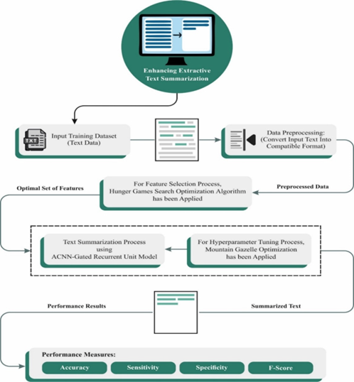
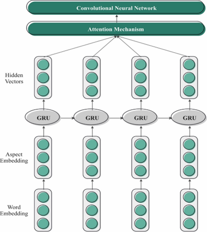
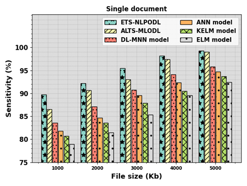
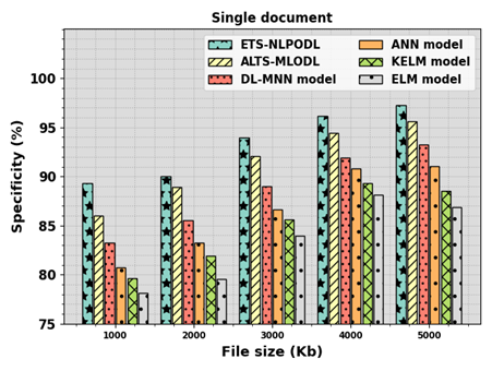
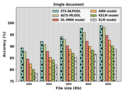
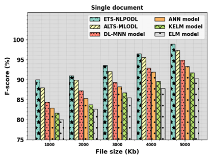
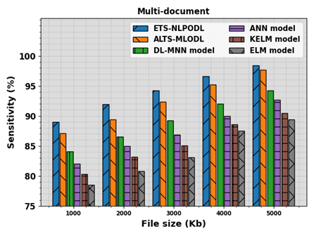
Natural language processing (NLP) performs a vital function in text summarization, a task targeted at refining the crucial information from the massive quantity of textual data. NLP methods allow computers to comprehend and process human language, permitting the development of advanced summarization methods. Text summarization includes the automatic generation of a concise and coherent summary of a specified document or collection of documents. Extracting significant insights from text data is crucial as it provides advanced solutions to end-users and business organizations. Automatic text summarization (ATS) computerizes text summarization by decreasing the initial size of the text without the loss of main data features. Deep learning (DL) approaches exhibited significant performance in abstractive and extractive summarization tasks. This research designed an extractive text summarization using NLP with an optimal DL (ETS-NLPODL) model. The major goal of the ETS-NLPODL technique was to exploit feature selection with a hyperparameter-tuned DL model for summarizing the text. In the ETS-NLPODL technique, an initial step of data preprocessing was involved to convert the input text into a compatible format. Next, a feature extraction process was carried out and the optimal set of features was chosen by the hunger games search optimization (HGSO) algorithm. For text summarization, the ETS-NLPODL model used an attention-based convolutional neural network with a gated recurrent unit (ACNN-GRU) model. Finally, the mountain gazelle optimization (MGO) algorithm was employed for the optimal hyperparameter selection of the ACNN-GRU model. The experimental results of the ETS-NLPODL system were examined under the benchmark dataset. The experimentation outcomes pointed out that the ETS-NLPODL technique gained better performance over other methods concerning diverse performance measures.
- text summarization,
- natural language processing,
- mountain gazelle optimization,
- feature extraction,
- deep learning
Citation: Abdulkhaleq Q. A. Hassan, Badriyya B. Al-onazi, Mashael Maashi, Abdulbasit A. Darem, Ibrahim Abunadi, Ahmed Mahmud. Enhancing extractive text summarization using natural language processing with an optimal deep learning model[J]. AIMS Mathematics, 2024, 9(5): 12588-12609. doi: 10.3934/math.2024616

Related Papers:

Abstract

Natural language processing (NLP) performs a vital function in text summarization, a task targeted at refining the crucial information from the massive quantity of textual data. NLP methods allow computers to comprehend and process human language, permitting the development of advanced summarization methods. Text summarization includes the automatic generation of a concise and coherent summary of a specified document or collection of documents. Extracting significant insights from text data is crucial as it provides advanced solutions to end-users and business organizations. Automatic text summarization (ATS) computerizes text summarization by decreasing the initial size of the text without the loss of main data features. Deep learning (DL) approaches exhibited significant performance in abstractive and extractive summarization tasks. This research designed an extractive text summarization using NLP with an optimal DL (ETS-NLPODL) model. The major goal of the ETS-NLPODL technique was to exploit feature selection with a hyperparameter-tuned DL model for summarizing the text. In the ETS-NLPODL technique, an initial step of data preprocessing was involved to convert the input text into a compatible format. Next, a feature extraction process was carried out and the optimal set of features was chosen by the hunger games search optimization (HGSO) algorithm. For text summarization, the ETS-NLPODL model used an attention-based convolutional neural network with a gated recurrent unit (ACNN-GRU) model. Finally, the mountain gazelle optimization (MGO) algorithm was employed for the optimal hyperparameter selection of the ACNN-GRU model. The experimental results of the ETS-NLPODL system were examined under the benchmark dataset. The experimentation outcomes pointed out that the ETS-NLPODL technique gained better performance over other methods concerning diverse performance measures.

References

[1]	M. Yadav, R. Katarya, A Systematic Survey of Automatic Text Summarization Using Deep Learning Techniques, In Modern Electronics Devices and Communication Systems: Select Proceedings of MEDCOM 2021, 397–405. Singapore: Springer Nature Singapore, 2023. https://doi.org/10.1007/978-981-19-6383-4_31
[2]	Y. M. Wazery, M. E. Saleh, A. Alharbi, A. A. Ali, Abstractive Arabic text summarization based on deep learning, Comput. Intel. Neurosci., 2022. https://doi.org/10.1155/2022/1566890 doi: 10.1155/2022/1566890
[3]	P. J. Goutom, N. Baruah, P. Sonowal, An abstractive text summarization using deep learning in Assamese, Int. J. Inf. Technol., 2023, 1–8. https://doi.org/10.1007/s41870-023-01279-7 doi: 10.1007/s41870-023-01279-7
[4]	V. L. Sireesha, Text Summarization for Resource-Poor Languages: Datasets and Models for Multiple Indian Languages (Doctoral dissertation, International Institute of Information Technology Hyderabad), 2023.
[5]	S. Dhankhar, M. K. Gupta, Automatic Extractive Summarization for English Text: A Brief Survey. In Proceedings of Second Doctoral Symposium on Computational Intelligence: DoSCI 2021, 183–198. Singapore: Springer Singapore, 2021. https://doi.org/10.1007/978-981-16-3346-1_15
[6]	B. Shukla, S. Gupta, A. K. Yadav, D. Yadav, Text summarization of legal documents using reinforcement learning: A study, In Intelligent Sustainable Systems: Proceedings of ICISS 2022, 403–414. Singapore: Springer Nature Singapore, 2022. https://doi.org/10.1007/978-981-19-2894-9_30
[7]	B. Baykara, T. Güngör, Turkish abstractive text summarization using pretrained sequence-to-sequence models, Nat. Lang. Eng., 29 (2023), 1275–1304. https://doi.org/10.1017/S1351324922000195 doi: 10.1017/S1351324922000195
[8]	M. Bani-Almarjeh, M. B. Kurdy, Arabic abstractive text summarization using RNN-based and transformer-based architectures, Inform. Process. Manag., 60 (2023), 103227. https://doi.org/10.1016/j.ipm.2022.103227 doi: 10.1016/j.ipm.2022.103227
[9]	H. Aliakbarpour, M. T. Manzuri, A. M. Rahmani, Improving the readability and saliency of abstractive text summarization using a combination of deep neural networks equipped with auxiliary attention mechanisms, J. Supercomput., 2022, 1–28.
[10]	S. N. Turky, A. S. A. Al-Jumaili, R. K. Hasoun, Deep learning based on different methods for text summary: A survey, J. Al-Qadisiyah Comput. Sci. Math., 13 (2021), 26. https://doi.org/10.29304/jqcm.2021.13.1.766 doi: 10.29304/jqcm.2021.13.1.766
[11]	G. A. Babu, S. Badugu, Deep learning based sequence to sequence model for abstractive Telugu text summarization, Multimed. Tools Appl., 82 (2023), 17075–17096. https://doi.org/10.1007/s11042-022-14099-x doi: 10.1007/s11042-022-14099-x
[12]	S. A. Tripathy, A. Sharmila, Abstractive method-based text summarization using bidirectional long short-term memory and pointer generator mode, J. Appl. Res. Technol., 21 (2023), 73–86. https://doi.org/10.22201/icat.24486736e.2023.21.1.1446 doi: 10.22201/icat.24486736e.2023.21.1.1446
[13]	N. Shafiq, I. Hamid, M. Asif, Q. Nawaz, H. Aljuaid, H. Ali, Abstractive text summarization of low-resourced languages using deep learning, PeerJ Comput. Sci., 9 (2023), e1176. https://doi.org/10.7717/peerj-cs.1176 doi: 10.7717/peerj-cs.1176
[14]	R. Karmakar, K. Nirantar, P. Kurunkar, P. Hiremath, D. Chaudhari, Indian regional language abstractive text summarization using attention-based LSTM neural network, In 2021 International Conference on Intelligent Technologies (CONIT), 1–8, IEEE, 2021. https://doi.org/10.1109/CONIT51480.2021.9498309
[15]	R. Rani, D. K. Lobiyal, Document vector embedding based extractive text summarization system for Hindi and English text, Appl. Intell., 2022, 1–20. https://doi.org/10.1007/s10489-021-02871-9 doi: 10.1007/s10489-021-02871-9
[16]	W. Etaiwi, A. Awajan, SemG-TS: Abstractive Arabic text summarization using semantic graph embedding, Mathematics, 10 (2022), 3225. https://doi.org/10.3390/math10183225 doi: 10.3390/math10183225
[17]	R. T. AlTimimi, F. H. AlRubbiay, Multilingual text summarization using deep learning, Int. J. Eng. Adv. Technol., 7 (2021), 29–39. https://doi.org/10.31695/IJERAT.2021.3712 doi: 10.31695/IJERAT.2021.3712
[18]	S. V. Moravvej, A. Mirzaei, M. Safayani, Biomedical text summarization using conditional generative adversarial network (CGAN), arXiv preprint arXiv: 2110.11870, 2021.
[19]	A. Al Abdulwahid, Software solution for text summarisation using machine learning based Bidirectional Encoder Representations from Transformers algorithm, IET SOFTWARE, 2023. https://doi.org/10.1049/sfw2.12098 doi: 10.1049/sfw2.12098
[20]	B. Muthu, S. Cb, P. M. Kumar, S. N. Kadry, C. H. Hsu, O. Sanjuan, et al., A framework for extractive text summarization based on deep learning modified neural network classifier, ACM T. Asian Low-Reso., 20 (2021), 1–20. https://doi.org/10.1145/3392048 doi: 10.1145/3392048
[21]	D. Izci, S. Ekinci, E. Eker, M. Kayri, Augmented hunger games search algorithm using logarithmic spiral opposition-based learning for function optimization and controller design, J. King Saud University-Eng. Sci., 2022. https://doi.org/10.1016/j.jksues.2022.03.001 doi: 10.1016/j.jksues.2022.03.001
[22]	M. Mafarja, T. Thaher, M. A. Al-Betar, J. Too, M. A. Awadallah, I. Abu Doush, et al., Classification framework for faulty-software using enhanced exploratory whale optimizer-based feature selection scheme and random forest ensemble learning, Appl. Intell., 2023, 1–43. https://doi.org/10.1007/s10489-022-04427-x doi: 10.1007/s10489-022-04427-x
[23]	B. Liu, J. Xu, W. Xia, State-of-Health Estimation for Lithium-Ion Battery Based on an Attention-Based CNN-GRU Model with Reconstructed Feature Series, Int. J. Energy Res., 2023. https://doi.org/10.1155/2023/8569161 doi: 10.1155/2023/8569161
[24]	P. Sarangi, P. Mohapatra, Evolved opposition-based Mountain Gazelle Optimizer to solve optimization problems, J. King Saud Univ-Com., 2023, 101812. https://doi.org/10.1016/j.jksuci.2023.101812 doi: 10.1016/j.jksuci.2023.101812
[25]	H. J. Alshahrani, K. Tarmissi, A. Yafoz, A. Mohamed, M. A. Hamza, I. Yaseen, et al., Applied linguistics with mixed leader optimizer based English text summarization model, Intell. Autom. Soft Co., 36 (2023). https://doi.org/10.32604/iasc.2023.034848 doi: 10.32604/iasc.2023.034848

Reader Comments

Your name:*

Email:*
© 2024 the Author(s), licensee AIMS Press. This is an open access article distributed under the terms of the Creative Commons Attribution License (http://creativecommons.org/licenses/by/4.0)