Neighbor event-triggered adaptive distributed control for multiagent systems with dead-zone inputs

Xiaohang Su; Peng Liu; Haoran Jiang; Xinyu Yu; Xiaohang Su; Peng Liu; Haoran Jiang; Xinyu Yu

doi:10.3934/math.2024491

AIMS Mathematics

2024, Volume 9, Issue 4: 10031-10049. doi: 10.3934/math.2024491

Previous Article Next Article

Research article

Neighbor event-triggered adaptive distributed control for multiagent systems with dead-zone inputs

School of Automation, Guangdong University of Technology, Guangzhou 510006, China

Received: 27 December 2023 Revised: 10 February 2024 Accepted: 19 February 2024 Published: 13 March 2024
MSC : 93B52, 93C95, 93D05

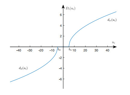
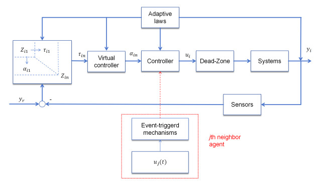
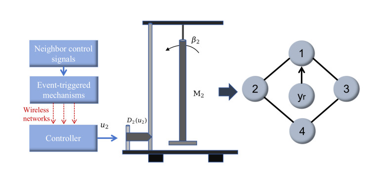
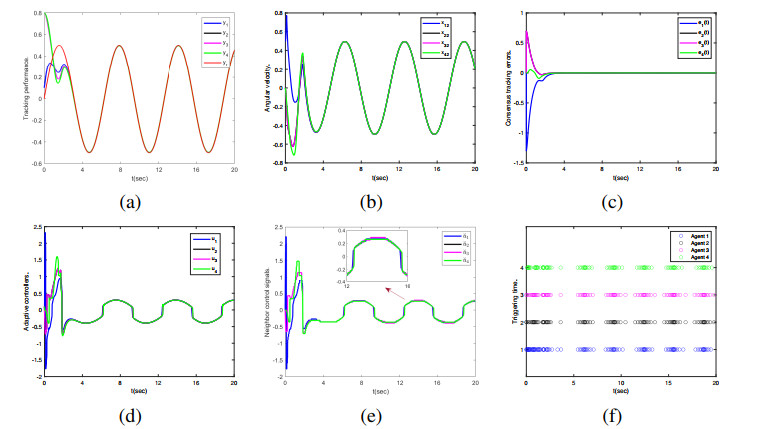
The paper focused on the distributed tracking problem for a specific class of multi-agent systems, characterized by bandwidth constraint and dead zone actuators, where the bandwidth limitations exist in neighbor agents and the dead zone nonlinearity refers to a generalized mathematical model. Initially, a series of event-triggered mechanisms with relative thresholds were established for neighbor agents, ensuring that control signals were transmitted only when necessary. Next, the generalized dead zone models were decomposed into two parts: indefinite terms with control coefficients and disturbance-like terms, resulting in unpredictability and damaging effects. Subsequently, based on the backstepping procedure, final consensus controllers with multiple polynomial compensators were constructed. These controllers offset the coupling coefficients caused by event-triggered mechanisms and dead zone non-smooth. Stability analysis was given to substantiate the theoretical correctness of this method and support the claim of Zeno behavior avoidance. Finally, simulation studies were performed for the feasibility of our proposed methodology.

Keywords:

Citation: Xiaohang Su, Peng Liu, Haoran Jiang, Xinyu Yu. Neighbor event-triggered adaptive distributed control for multiagent systems with dead-zone inputs[J]. AIMS Mathematics, 2024, 9(4): 10031-10049. doi: 10.3934/math.2024491

Related Papers:

[1]	Zeshan Qiu . Fourth-order high-precision algorithms for one-sided tempered fractional diffusion equations. AIMS Mathematics, 2024, 9(10): 27102-27121. doi: 10.3934/math.20241318
[2]	Zunyuan Hu, Can Li, Shimin Guo . Fast finite difference/Legendre spectral collocation approximations for a tempered time-fractional diffusion equation. AIMS Mathematics, 2024, 9(12): 34647-34673. doi: 10.3934/math.20241650
[3]	Ridha Dida, Hamid Boulares, Bahaaeldin Abdalla, Manar A. Alqudah, Thabet Abdeljawad . On positive solutions of fractional pantograph equations within function-dependent kernel Caputo derivatives. AIMS Mathematics, 2023, 8(10): 23032-23045. doi: 10.3934/math.20231172
[4]	Muhammad Tariq, Sotiris K. Ntouyas, Hijaz Ahmad, Asif Ali Shaikh, Bandar Almohsen, Evren Hincal . A comprehensive review of Grüss-type fractional integral inequality. AIMS Mathematics, 2024, 9(1): 2244-2281. doi: 10.3934/math.2024112
[5]	Sadia Arshad, Iram Saleem, Ali Akgül, Jianfei Huang, Yifa Tang, Sayed M Eldin . A novel numerical method for solving the Caputo-Fabrizio fractional differential equation. AIMS Mathematics, 2023, 8(4): 9535-9556. doi: 10.3934/math.2023481
[6]	H. H. G. Hashem, Hessah O. Alrashidi . Qualitative analysis of nonlinear implicit neutral differential equation of fractional order. AIMS Mathematics, 2021, 6(4): 3703-3719. doi: 10.3934/math.2021220
[7]	Ahmed Morsy, Kottakkaran Sooppy Nisar, Chokkalingam Ravichandran, Chandran Anusha . Sequential fractional order Neutral functional Integro differential equations on time scales with Caputo fractional operator over Banach spaces. AIMS Mathematics, 2023, 8(3): 5934-5949. doi: 10.3934/math.2023299
[8]	Ritu Agarwal, Mahaveer Prasad Yadav, Dumitru Baleanu, S. D. Purohit . Existence and uniqueness of miscible flow equation through porous media with a non singular fractional derivative. AIMS Mathematics, 2020, 5(2): 1062-1073. doi: 10.3934/math.2020074
[9]	Djamila Chergui, Taki Eddine Oussaeif, Merad Ahcene . Existence and uniqueness of solutions for nonlinear fractional differential equations depending on lower-order derivative with non-separated type integral boundary conditions. AIMS Mathematics, 2019, 4(1): 112-133. doi: 10.3934/Math.2019.1.112
[10]	Naimi Abdellouahab, Keltum Bouhali, Loay Alkhalifa, Khaled Zennir . Existence and stability analysis of a problem of the Caputo fractional derivative with mixed conditions. AIMS Mathematics, 2025, 10(3): 6805-6826. doi: 10.3934/math.2025312

Abstract

1. Introduction

In this paper, we consider the Cauchy problem for the following two-dimensional inhomogeneous incompressible viscoelastic rate-type fluids with stress-diffusion:

$\begin{equation} \begin{cases} \rho_t+u\cdot\nabla\rho = 0, \qquad (t, x)\in\mathbb{R}^+\times\mathbb{R}^2, \\ \rho(u_t+u\cdot\nabla u)-\Delta u+\nabla P+\sigma \mathrm{div}\, (\nabla b\otimes\nabla b-\frac{1}{2}|\nabla b|^2\mathbb{I}) = 0, \\ b_t+u\cdot\nabla b+\frac{1}{\nu}(e'(b)-\sigma\Delta b) = 0, \\ \mathrm{div}\, u = 0, \\ (\rho, u, b)(t, x)|_{t = 0} = (\rho_0, u_0, b_0)(x), \end{cases} \end{equation}$

(1.1)

where the unknowns $\rho = \rho(x, t)$ , $u = (u^1(x, t), u^2(x, t))$ and $b = b(x, t)$ stand for the density, velocity of the fluid and the spherical part of the elastic strain, respectively. $P$ is a scalar pressure function, which guarantees the divergence-free condition of the velocity field. The coefficients $\nu$ and $\sigma$ are two positive constants. In addition, we suppose that $e(\cdot)$ is a smooth convex function about $b$ and $e(0)\leq0$ , $e'(0) = 0$ , $e''(b)\leq C_0$ , where $C_0$ is a positive constant depending on the initial data. The class of fluids is the elastic response described by a spherical strain ^[3]. Compared with ^[3], we have added the divergence-free condition to investigate the effect of density on viscoelastic rate-type fluids, while the divergence-free condition is for computational convenience.

It is easy to observe that for $\sigma = 0$ , the system (1.1) degenerates two distinct systems involving the inhomogeneous Navier-Stokes equation for the fluid and a transport equation with damped $e'(b)$ . Numerous researchers have extensively studied the well-posedness concern regarding the inhomogeneous Navier-Stokes equations; see ^{[1,7,8,9,11,14]} and elsewhere. However, the transport equation has a greater effect on the regularity of density than on that of velocity. Additionally, due to the presence of the damped term $e'(b)$ , the initial elasticity in system (1.1) exhibits higher regularity compared to the initial velocity.

In the case where $\sigma > 0$ , system (1.1) resembles the inhomogeneous magnetohydrodynamic (MHD) equations, with $b$ as a scalar function in (1.1) that does not satisfy the divergence condition found in MHD equations. It is essential to highlight that the system (1.1) represents a simplified model, deviating from standard viscoelastic rate-type fluid models with stress-diffusion to facilitate mathematical calculations. Related studies on system (1.1) can be found in ^[3,4,15]. In particular, Bulíček, Málek, and Rodriguez in ^[5] established the well-posedness of a 2D homogeneous system (1.1) in Sobolev space. Our contribution lies in incorporating the density equation into this established framework.

Inspired by ^[11,18], we initially establish a priori estimates for the system (1.1). Subsequently, by using a Friedrich's method and the compactness argument, we obtain the existence and uniqueness of the solutions. Our main result is as follows:

Theorem 1.1. Let the initial data $(\rho_0, u_0, b_0)$ satisfy

$\begin{align} 0 < m < \rho_0(x) < M < \infty, \quad (u_{0}, b_{0})\in H^{1}(\mathbb{R}^{2})\times H^{2}(\mathbb{R}^{2}), \, \, e(b_0)\in L^1(\mathbb{R}^{2}), \end{align}$

(1.2)

where $m, M$ are two given positive constants with $m < M$ . Then system (1.1) has a global solution $(\rho, u, b)$ such that, for any given $T > 0$ , $(t, x)\in[0, T)\times\mathbb{R}^2$ ,

$\begin{align*} & \qquad\qquad\qquad m < \rho(t, x) < M, \\ &u\in L^\infty(0, T; H^1(\mathbb{R}^2))\cap L^{2}(0, T; H^2(\mathbb{R}^2)), \quad \partial_tu\in L^\infty(0, T; L^2(\mathbb{R}^2))\cap L^{2}(0, T; H^1(\mathbb{R}^2)), \\ &b\in L^\infty(0, T; H^2(\mathbb{R}^2))\cap L^{2}(0, T; H^3(\mathbb{R}^2)), \quad \partial_tb\in L^\infty(0, T; H^1(\mathbb{R}^2))\cap L^{2}(0, T; H^2(\mathbb{R}^2)). \end{align*}$

Moreover, if $\nabla\rho_0\in L^4(\mathbb{R}^2)$ , then the solution is unique.

Remark 1.1. Compared to the non-homogeneous MHD equations, handling the damping term $e'(b)$ poses a challenge, so that we cannot obtain the time-weighted energy of the velocity field. To explore the uniqueness of the solution, it is necessary to improve the regularity of the initial density data.

The key issue to prove the global existence part of Theorem 1.1 is establishing the a priori $L^\infty(0, T; H^1(\mathbb{R}^2))$ estimate on $(u, \nabla b)$ for any positive time $T$ . We cannot directly estimate the $L^2$ estimate of $(u, b)$ , which mainly occurs in the velocity term $\mathrm{div}\, (\nabla b\otimes\nabla b-\frac{1}{2}\left|\nabla b\right|^2\mathbb{I})$ . Therefore, we need to estimate the $L^2$ of the $\nabla b$ equation. Afterwards, the $L^2$ estimation of equation $b$ was affected by a damping term $e'(b)$ , so we made an $L^2$ estimation of equation $e'(b)$ . Finally, to show the $L^\infty(0, T; H^1(\mathbb{R}^2))$ of $u$ , we also need an estimate of the second derivative of $b$ . In summary, we found that the initial value of the $b$ equation needs to be one derivative higher than the initial value of the $u$ equation.

Concerning the uniqueness of the strong solutions, a common approach is to consider the difference equations between two solutions and subsequently derive some energy estimates for the resulting system differences based on the fundamental natural energy of the system. However, for system (1.1), the presence of a damping term $e'(b)$ of the equation $b$ and density equation prevents the calculation of the time-weighted energy of the velocity field. To research the solution's uniqueness, we need to enhance the regularity of the initial density data.

The paper is structured as follows: Section 2 presents prior estimates for system (1.1). In Section 3, we establish the existence and uniqueness of Theorem 1.1.

2. A priori estimates

Proposition 2.1. Assume that $m, M$ are two given positive constants and $0 < m \leq M < \infty$ , the initial data $\rho_{0}$ satisfies $0 < m\le \rho_{0}\le M < +\infty$ , and the initial data $(\sqrt{\rho_0}u_0, \nabla b_0)\in L^{2}(\mathbb{R}^{2})\times L^{2}(\mathbb{R}^{2})$ . Let $(\rho, u, b)$ be a smooth solution of system (1.1), then there holds for any $t > 0$ ,

$\begin{align} 0 < m\le \rho(t)\le M < +\infty, \end{align}$

(2.1)

$\begin{align} \|(\sqrt{\rho}u, \nabla b, u)(t)\| _{L^2}^2 +\int_{0}^{t} \|(\nabla u, \nabla ^{2} b )\|_{L^{2}}^{2}\mathrm{d}\tau\leq C{\Vert (\sqrt{\rho_0}u_0 , \nabla b_0 )\Vert_{L^2}^2}, \end{align}$

(2.2)

where C is a constant depending only on $\sigma$ , $\nu$ .

Proof. First, any Lebesgue norm of $\rho_0$ is preserved through the evolution, and $0 < m\le \rho(t)\le M < +\infty$ .

To prove (2.2), taking the $L^{2}$ inner product of the second equation of (1.1) with $u$ and integrating by parts, then we obtain

$\begin{align} \frac{1}{2}\frac{\mathrm{d}}{\mathrm{d}t} \|\sqrt{\rho}u\|_{L^{2}}^{2} + \|\nabla u\|_{L^{2}}^{2} = -\sigma \int_{\mathbb{R}^2} \Delta b\nabla b\cdot u \mathrm{d} x, \end{align}$

(2.3)

where we used the fact that

$\begin{align*} \mathrm{div}\, (\nabla b\otimes\nabla b-\frac{1}{2}\left|\nabla b\right|^2\mathbb{I}) = \Delta b \nabla b. \end{align*}$

Multiplying the third equation of (1.1) by $-\sigma\Delta b$ and integrating by parts, we obtain

$\begin{align} \frac{\sigma}{2} \frac{\mathrm{d}}{\mathrm{d}t} \|\nabla b\|_{L^{2}}^{2}+\frac{\sigma^{2}}{\nu} \|\Delta b\|_{L^{2}}^2 - \frac{\sigma^2}{\nu}\int_{\mathbb{R}^{2}} e'(b)\Delta b\mathrm{d}x = \sigma\int_{\mathbb{R}^{2}} u\cdot\nabla b\Delta b\mathrm{d}x . \end{align}$

(2.4)

Thanks to the convexity of $e(b)$ , we know

$\begin{align} -\frac{\sigma^{2}}{\nu}\int_{\mathbb{R}^2} e'(b)\Delta b\mathrm{d}x = \frac{\sigma^2}{\nu}\int_{\mathbb{R}^2} \nabla (e'(b))\nabla b\mathrm{d}x = \frac{\sigma ^{2}}{\nu} \int_{\mathbb{R}^2} e''(b){\left|\nabla b\right|}^2\mathrm{d}x\geq0. \end{align}$

(2.5)

By inserting (2.5) into (2.4), combining the result with (2.3), one yields

$\begin{align*} \frac{\mathrm{d}}{\mathrm{d}t} \|(\sqrt{\rho}u, \nabla b)\|_{L^{2}}^{2}+ \|\nabla u\|_{L^{2}}^{2}+C \|\Delta b\|_{L^{2}}^{2}\leq 0. \end{align*}$

Integrating it with respect to time, we have

$\begin{align} \|(\sqrt{\rho}u, \nabla b )(t)\| _{L^{2}}^{2} +\int_0^t {\Vert (\nabla u, \nabla ^2 b )\Vert_{L^2}^2} \mathrm{d} \tau \leq C{\Vert (\sqrt{\rho_0}u_0 , \nabla b_0 )\Vert_{L^2}^2}. \end{align}$

(2.6)

On the other hand, applying $0 < m\le \rho \le M < + \infty$ , which together with (2.6) implies

$\begin{equation*} \|u\|_{L^\infty (L^2)}^2\leq m^{-1}\|\sqrt{\rho}u\|_{L^\infty(L^2)}^2\le C{\Vert (\sqrt{\rho_0}u_0 , \nabla b_0 )\Vert_{L^2}^2}, \end{equation*}$

which, along with inequality (2.6), yields (2.2). □

Proposition 2.2. Under the assumptions of Proposition 2.1, the corresponding solution ( $\rho$ , u, b) of the system (1.1) admits the following bound for any $t > 0$ :

$\begin{equation} \Vert (\nabla u, \nabla ^2 b, \nabla b, b ) \Vert_{L^2}^2 + \int_0 ^t \Vert (\nabla ^2 u, \nabla ^3 b, \sqrt{\rho} u_ \tau , b_ \tau, u_ \tau ) \Vert_{L^2}^2 \mathrm{d} \tau \le C, \end{equation}$

(2.7)

where $C$ is a positive constant depending on $m$ , $M$ , $u_0$ , $\rho_0$ , and $\nabla b_0$ .

Proof. First, we obtain by taking $L^2$ inner product of $(1.1)_3$ with $e'(b)$ that

$\begin{align*} &\frac{\mathrm{d}}{\mathrm{d}t} \int_{\mathbb{R}^2} e(b) \mathrm{d} x + {\frac{1}{\nu}}{\Vert e'(b) \Vert_{L^2}^2} \\ & \le \Vert u \cdot \nabla b \Vert_{L^2} \Vert e'(b) \Vert_{L^2} + \frac{1}{4\nu} \Vert e'(b) \Vert_{L^2}^2 + C \Vert \Delta b \Vert_{L^2}^2 \\ & \le \frac{1}{2\nu} \Vert e'(b) \Vert_{L^2}^2 + C \Vert u \Vert_{L^4}^2 \Vert \nabla b \Vert_{L^4}^2 + C \Vert \Delta b \Vert_{L^2}^2 \\ & \le \frac{1}{2\nu} \Vert e'(b) \Vert_{L^2}^2 + C \Vert u \Vert_{L^2} \Vert \nabla u \Vert_{L^2} \Vert \nabla b \Vert_{L^2} \Vert \nabla^2 b \Vert_{L^2} + C \Vert \Delta b \Vert_{L^2}^2 \\ & \le \frac{1}{2\nu} \Vert e'(b) \Vert_{L^2}^2 + C ( \Vert \nabla u \Vert_{L^2}^2 + \Vert \nabla^2 b \Vert_{L^2}^2). \end{align*}$

Integrating with respect to time, we obtain

$\begin{equation} \|e(b) \|_{L^\infty(L^{1})} + {\Vert e'(b) \Vert_{L^2(L^2)}^2}\leq {\Vert (\sqrt{\rho_0}u_0 , \nabla b_0 )\Vert_{L^2}^2}+\|e(b_0) \|_{L^{1}}. \end{equation}$

(2.8)

Similarly, multiplying $(1.1)_3$ by $b$ , we have

$\begin{equation*} \frac{1}{2}\frac{\mathrm{d}}{\mathrm{d}t}\|b\|_{L^2}^2+\|\nabla b\|_{L^2}^2\leq C(\|b\|_{L^2}^2+\Vert e'(b) \Vert_{L^2}^2), \end{equation*}$

after using (2.8) and Grönwall's inequality, we obtain

$\begin{equation} b \in L^\infty(0, t;L^2(\mathbb{R}^2))\cap L^2(0, t;H^1(\mathbb{R}^2)). \end{equation}$

(2.9)

In the following, applying Laplace operator $\Delta$ to $(1.1) _3$ and multiplying the resulting equation by $\Delta b$ ; additionally, multiplying $(1.1)_2$ by $u_t$ and $(1.1)_3$ by $b_t$ , respectively, then integrating them on $\mathbb{R}^2$ and adding up all these results together, we obtain

$\begin{align} &\frac{1}{2} \frac{\mathrm{d}}{\mathrm{d}t} \int_{\mathbb{R}^2}(|\Delta b |^2+|\nabla u|^2+\frac{\sigma}{\nu}|\nabla b|^2)\mathrm{d}x + \int_{\mathbb{R}^2} (\rho |u_t|^2 + |b_t|^2 + \frac{\sigma}{\nu} | \nabla ^3 b|^2 ) \mathrm{d}x \\ & = -\int_{\mathbb{R}^2} {\rho u \cdot \nabla u \cdot u_t} \mathrm{d} x -\sigma \int_{\mathbb{R}^2} {\Delta b \nabla b \cdot u_t} \mathrm{d} x-\int_{\mathbb{R}^2} {u \cdot\nabla b b_t} \mathrm{d} x \\ & \quad - \frac{1}{\nu} \int_{\mathbb{R}^2} {e'(b) b_t} \mathrm{d} x- \int_{\mathbb{R}^2} \Delta (u\cdot \nabla b) \cdot\Delta b \mathrm{d} x -\frac{1}{\nu} \int_{\mathbb{R}^2} \Delta e'(b) \cdot\Delta b \mathrm{d} x \\ &\triangleq \sum\limits_{j = 1}^{6}I_j. \end{align}$

(2.10)

Utilizing Gagliardo-Nirenberg's, Hölder's, Young's inequalities (2.2), we estimate the first term as follows:

$\begin{align*} I_1 & \le {\Vert \sqrt{\rho} \Vert_{L^\infty}}{\Vert \sqrt{\rho} u_t \Vert_{L^2}}\| u\|_{L^4} \|\nabla u\|_{L^4}\\ &\le \frac{1}{16} \Vert \sqrt{\rho} u_t \Vert_{L^2}^2 + C \Vert u \Vert_{L^4}^2 \Vert \nabla u\Vert_{L^4}^2 \\ & \le \frac{1}{16} \Vert \sqrt{\rho} u_t \Vert_{L^2}^2 + C \Vert u \Vert_{L^2} {\Vert \nabla u \Vert_{L^2}^2 } {\Vert \nabla^2 u \Vert_{L^2}}\\ & \le \frac{1}{16} \Vert \sqrt{\rho} u_t \Vert_{L^2}^2 + \frac{1}{16} \Vert \nabla^2 u \Vert_{L^2}^2 + C \Vert \nabla u \Vert_{L^2}^4. \end{align*}$

Similarly, by direct calculations, the other terms can be bounded as

$\begin{align*} I_2 & \le \frac{1}{16} \Vert \sqrt{\rho} u_t \Vert_{L^2}^2 +\frac{\sigma}{8\nu}\Vert \nabla^3 b \Vert_{L^2} ^2 + C \Vert \nabla^2 b \Vert_{L^2}^4, \\ I_3 & \le \frac{1}{4} \Vert b_t \Vert_{L^2}^2 + C \Vert \nabla u \Vert_{L^2}^2 +C \|\nabla b\|_{L^2}^2\Vert \Delta b \Vert_{L^2}^2, \\ I_4 & \le \frac{1}{4} {\Vert b_t \Vert_{L^2}^2} + C {\Vert e'(b) \Vert_{L^2}^2}, \\ I_5&\le\frac{3\sigma}{16\nu} \Vert \nabla^3 b \Vert_{L^2}^2 + \frac{1}{16} \Vert \nabla^2 u \Vert_{L^2}^2 + C \Vert \nabla u \Vert_{L^2}^4 + C\Vert \nabla^2 b \Vert_{L^2} ^4, \\ I_6& \le \frac{3\sigma}{16\nu} \Vert \nabla^3 b \Vert_{L^2}^2 +C \|\nabla b\|_{L^2}^2. \end{align*}$

Next, according to the regularity theory of the Stokes system in Eq $(1.1)_2$ , it follows that

$\begin{align*} \Vert \nabla^2 u \Vert_{L^2}^2 & \le \Vert \rho u_t \Vert_{L^2}^2 + \Vert \rho u \cdot \nabla u \Vert_{L^2}^2 + \sigma \Vert \nabla b \Delta b \Vert_{L^2}^2\\ & \le \Vert \sqrt{\rho} u_t \Vert_{L^2}^2 +C \Vert \nabla u \Vert_{L^2}^2 \Vert \nabla^2 u \Vert_{L^2} + C\Vert \nabla^2 b \Vert_{L^2}^2 \Vert \nabla^3 b \Vert_{L^2}\\ & \le \Vert \sqrt{\rho} u_t \Vert_{L^2}^2 +\frac{1}{2} \Vert \nabla^2 u \Vert_{L^2}^2 + \frac{\sigma}{2\nu} \Vert \nabla^3 b \Vert_{L^2} ^2 +C (\Vert \nabla u \Vert_{L^2}^4 + \Vert \nabla^2 b \Vert_{L^2}^4), \end{align*}$

after multiplying by $\frac{1}{8}$ , we arrive at

$\begin{align} \frac{1}{16}\Vert \nabla^2 u \Vert_{L^2}^2 & \leq \frac{1}{8} \Vert \rho u_t \Vert_{L^2}^2 + \frac{\sigma}{16\nu} \Vert \nabla^3 b \Vert_{L^2}^2 +C( \Vert \nabla u \Vert_{L^2}^4 +\Vert \nabla^2 b \Vert_{L^2}^4). \end{align}$

(2.11)

Substituting the estimates $I_1-I_6$ into (2.10) and combining inequality (2.11), we have

$\begin{align*} &\frac{\mathrm{d}}{\mathrm{d}t} (\Vert (\nabla u, \nabla b, \nabla^2 b)\Vert_{L^2}^2 +1)+ \Vert( \sqrt{\rho} u_t, b_t, \nabla ^3 b, \nabla ^2 u) \Vert_{L^2}^2 \\ & \le C (\Vert (\nabla u, \nabla b, \nabla^2 b)\Vert_{L^2}^2 +1)\Vert (\nabla u, \nabla b, \nabla^2 b ) \Vert_{L^2}^2 + C \Vert e'(b) \Vert_{L^2}^2, \end{align*}$

which, along with Grönwall's inequality (2.2), (2.8), and (2.9), leads to

$\begin{equation} \Vert (\nabla u , \nabla b , \nabla^2 b) \Vert_{L^2}^2 + \int_{0}^{t} \Vert (\sqrt{\rho} u_\tau , b_\tau , \nabla ^3 b, \nabla ^2 u ) \Vert_{L^2}^2\mathrm{d}\tau \le C, \end{equation}$

(2.12)

which completes the proof of Proposition 2.2. □

Proposition 2.3. Under the assumptions of Proposition 2.2, there holds

$\begin{align} \Vert (\sqrt{\rho} u_t , b_t, \nabla b_t, u_t ) \Vert_{L^2}^2 + \int_{0}^{t} \Vert (\nabla u_ \tau , \nabla b_\tau , \Delta b_\tau ) \Vert_{L^2}^2 \mathrm{d} \tau \le C, \end{align}$

(2.13)

where $C$ is a positive constant depending on $m$ , $M$ , $u_0$ , $\rho_0$ and $b_0$ .

Proof. Taking the derivative of Eq $(1.1)_2$ with respect to time $t$ , then multiplying $u_t$ on both sides of the resulting equation and integrating by parts gives

$\begin{align} \frac{1}{2}\frac{\mathrm{d}}{\mathrm{d}t} \Vert \sqrt{\rho} u_t \Vert_{L^2}^2 + \Vert \nabla u_t \Vert_{L^2}^2 = & -\int_{\mathbb{R}^2} \rho _t u_t\cdot u_t \mathrm{d} x -\int_{\mathbb{R}^2} \rho _t u \cdot \nabla u \cdot u_t \mathrm{d} x -\int_{\mathbb{R}^2} \rho u_t\cdot \nabla u\cdot u_t \mathrm{d} x\\ &- \int_{\mathbb{R}^2} \sigma \Delta b_t \nabla b\cdot u_t \mathrm{d} x - \sigma \int_{\mathbb{R}^2} \Delta b \nabla b_t \cdot u_t \mathrm{d} x. \end{align}$

(2.14)

Next, we compute each term on the right-hand side of the equation above one by one using estimates (2.2) and (2.7). The bound of the first term has been estimated as

$\begin{align*} -\int_{\mathbb{R}^2} \rho _t u_t\cdot u_t \mathrm{d} x & = \int_{\mathbb{R}^2} \ \mathrm{div}\, {(\rho u )} u_t \cdot u_t \mathrm{d} x = -\int_{\mathbb{R}^2} 2 \rho u u_t \cdot \nabla u_t \mathrm{d} x \\ &\le C \Vert \rho \Vert_{L^\infty} \Vert u \Vert_{L^4} \Vert u_t \Vert_{L^4} \Vert \nabla u_t \Vert_{L^2} \\ &\le C \Vert u \Vert_{L^2}^ \frac{1}{2} \Vert \nabla u \Vert_{L^2}^ \frac{1}{2} \Vert \nabla u_t \Vert_{L^2}^ \frac{3}{2} \Vert u_t \Vert_{L^2}^ \frac{1}{2}\\& \le \frac{1}{10}\Vert \nabla u_t \Vert_{L^2}^2 + C \Vert \nabla u \Vert_{L^2}^ 2 \Vert u_t \Vert_{L^2}^2. \end{align*}$

By using Gagliardo-Nirenberg's, Hölder's, and Young's inequalities and (2.2), we have

$\begin{align*} &-\int_{\mathbb{R}^2} \rho _t u \cdot \nabla u\cdot u_t \mathrm{d} x = \int_{\mathbb{R}^2} \nabla \cdot(\rho u) u \cdot \nabla u \cdot u_t \mathrm{d} x\\ & = -\int_{\mathbb{R}^2}\rho u \cdot \nabla u \cdot \nabla u \cdot u_t\mathrm{d} x - \int_{\mathbb{R}^2} \rho u \cdot u \cdot \nabla ^2 u\cdot u_t \mathrm{d} x-\int_{\mathbb{R}^2} u \cdot\nabla u \cdot \rho u \cdot\nabla u_t \mathrm{d} x\\ &\leq \|\rho\|_{L^\infty}\big(\|u\|_{L^6}\|\nabla u\|_{L^3}^2\|u_t\|_{L^6}+\|u\|_{L^6}^2\|\nabla^2u\|_{L^2}\|u_t\|_{L^6}+\|u\|_{L^6}^2\|\nabla u\|_{L^6}\|\nabla u_t\|_{L^2}\big)\\ & \le C \Vert u \Vert_{L^2}^\frac{1}{3} \Vert \nabla u \Vert_{L^2}^2 \Vert \nabla^2 u \Vert_{L^2}^\frac{2}{3} \Vert u_t \Vert_{L^2}^\frac{1}{3} \Vert \nabla u_t \Vert_{L^2}^\frac{2}{3}+ C \Vert u \Vert_{L^2}^\frac{2}{3} \Vert \nabla u \Vert_{L^2}^\frac{4}{3} \Vert \nabla^2 u \Vert_{L^2} \Vert u_t \Vert_{L^2}^ \frac{1}{3} \Vert \nabla u_t \Vert_{L^2}^\frac{2}{3}\\ &\ \quad + C \Vert u \Vert_{L^2}^\frac{2}{3} \Vert \nabla u \Vert_{L^2}^\frac{5}{3} \Vert \nabla^2 u \Vert_{L^2}^\frac{2}{3} \Vert \nabla u_t \Vert_{L^2} \\ &\le \frac{1}{10}\Vert \nabla u_t \Vert_{L^2}^2 + C \Vert \nabla^2 u \Vert_{L^2}^2 + C \|\nabla u\|_{L^2}^2\Vert u_t \Vert_{L^2}^2 . \end{align*}$

Similarly,

$\begin{align*} -\int_{\mathbb{R}^2} \rho u_t \cdot \nabla u \cdot u_t \mathrm{d} x \le C \Vert \rho \Vert_{L^\infty} \Vert \nabla u \Vert_{L^2} \Vert u_t \Vert_{L^4}^2 \le \frac{1}{10}\Vert \nabla u_t \Vert_{L^2}^2 + C\|\nabla u\|_{L^{2}}^2 \Vert u_t \Vert_{L^2}^2 \end{align*}$

and

$\begin{align*} &\ -\int_{\mathbb{R}^2} \sigma \Delta b_t \nabla b\cdot u_t \mathrm{d} x - \sigma \int_{\mathbb{R}^2} \Delta b \nabla b_t \cdot u_t \mathrm{d} x\\ &\le C \Vert \Delta b_t \Vert_{L^2} \Vert \nabla b \Vert_{L^4} \Vert u_t \Vert_{L^4} + C \Vert \Delta b \Vert_{L^4} \Vert \nabla b_t \Vert_{L^2} \Vert u_t \Vert_{L^4} \\ & \le C \Vert \Delta b_t \Vert_{L^2} \Vert \nabla b \Vert_{L^2}^ \frac{1}{2} \Vert \Delta b \Vert_{L^2}^\frac{1}{2} \Vert u_t \Vert_{L^2}^\frac{1}{2} \Vert \nabla u_t \Vert_{L^2}^\frac{1}{2} + C \Vert \Delta b \Vert_{L^2}^\frac{1}{2} \Vert \nabla^3 b \Vert_{L^2}^\frac{1}{2} \Vert \nabla b_t \Vert_{L^2} \Vert u_t \Vert_{L^2}^\frac{1}{2} \Vert \nabla u_t \Vert_{L^2} ^\frac{1}{2} \\ & \le \frac{\sigma}{16\nu}\Vert \nabla b_t \Vert_{L^2} ^2 + \frac{\sigma}{16\nu}\Vert \Delta b_t \Vert_{L^2} ^2 + \frac{1}{10}\Vert \nabla u_t \Vert_{L^2} ^2+ C(\|\nabla b\|_{L^2}^2+ \Vert \nabla^3 b \Vert_{L^2} ^2) \|\nabla^2 b\|_{L^2}^2 \Vert u_t \Vert_{L^2} ^2. \end{align*}$

Inserting these estimates into (2.14), we have

$\begin{align} \frac{\mathrm{d}}{\mathrm{d}t} \Vert \sqrt{\rho} u_t \Vert_{L^2}^2 + &\frac{8}{5}\Vert \nabla u_t \Vert_{L^2}^2\le \frac{\sigma}{8\nu}\Vert( \nabla b_t, \Delta b_t)\Vert_{L^2}^2+ C \Vert \nabla^2 u\Vert_{L^2}^2\\ & \qquad\qquad\qquad+C\|(\nabla u, \nabla^2 b, \nabla^3 b)\|_{L^2}^2\|u_t\|_{L^2}^2. \end{align}$

(2.15)

Now we turn to the $b$ equation of (1.1). Differentiating $(1.1)_3$ with respect to $t$ , we obtain

$\begin{equation*} b_{tt} + u_t \cdot \nabla b + u \cdot \nabla b_t + \frac{1}{\nu}(e''(b) b_t - \sigma \Delta b_t ) = 0. \end{equation*}$

Multiplying it by $b_t$ and $-\Delta b_t$ , integrating the resulting equation, and summing up these results, due to the divergence-free condition $\mathrm{div}\, u = 0$ , we obtain

$\begin{equation} \begin{split} & \frac{1}{2}\frac{\mathrm{d}}{\mathrm{d}t} \Vert( b_t, \nabla b_t )\Vert_{L^2}^2 + \frac{\sigma}{\nu} \Vert (\nabla b_t, \Delta b_t) \Vert_{L^2}^2 + \frac{1}{\nu} \int_{\mathbb{R}^2} e''(b) (b_t)^2 \mathrm{d} x \\ & = \int_{\mathbb{R}^2} u_t\cdot b \cdot \nabla b_t \mathrm{d} x +\int_{\mathbb{R}^2} u_t \cdot \nabla b\cdot \Delta b_t \mathrm{d} x + \int_{\mathbb{R}^2} u \cdot\nabla b_t \cdot\Delta b_t \mathrm{d} x +\frac{1}{\nu} \int_{\mathbb{R}^2} e''(b) b_t \cdot \Delta b_t \mathrm{d} x \\ & \le \Vert u_t \Vert_{L^4} \Vert b \Vert_{L^4} \Vert \nabla b_t \Vert_{L^2} + \Vert u_t \Vert_{L^4} \Vert \nabla b \Vert_{L^4} \Vert \Delta b_t \Vert_{L^2}+\Vert u \Vert_{L^4} \Vert \nabla b _t \Vert_{L^4} \Vert \Delta b_t \Vert_{L^2}+ C\Vert b_t \Vert_{L^2} \Vert \Delta b_t \Vert_{L^2} \\ & \le \frac{\sigma }{4\nu } \Vert \nabla b_t \Vert_{L^2}^2 + \Vert u_t \Vert_{L^2} \Vert \nabla u_t \Vert_{L^2} \Vert b \Vert_{L^2} \Vert \nabla b \Vert_{L^2} +\frac{\sigma}{8\nu} \Vert \Delta b_t \Vert_{L^2} ^2 + \Vert u_t \Vert_{L^2} \Vert \nabla u_t \Vert_{L^2} \Vert \nabla b \Vert_{L^2} \Vert \Delta b \Vert_{L^2} \\ &\quad +\frac{\sigma}{8\nu} \Vert \Delta b_t \Vert_{L^2} ^2 + C \Vert u \Vert_{L^ 2 } \Vert \nabla u \Vert_{L^2}\Vert \nabla b_t \Vert_{L^2} \Vert \nabla^2 b_t \Vert_{L^2} + \frac{\sigma}{8\nu} \Vert \Delta b_t \Vert_{L^2}^2 + C \Vert b_t \Vert_{L^2} ^2 \\ & \le \frac{\sigma }{4\nu} \Vert \nabla b_t \Vert_{L^2}^2 +\frac{\sigma}{2\nu} \Vert \Delta b_t \Vert_{L^2}^2 + \frac{1}{2} \Vert \nabla u_t \Vert_{L^2}^2 +C(\|\nabla b\|_{L^2}^2+\|\Delta b\|_{L^2}^2)\Vert u_t \Vert_{L^2} ^2+ C \Vert b_t \Vert_{L^2} ^2 \\ & \quad+C\|\nabla u\|_{L^2}^2\|\nabla b_t\|_{L^2}^2. \end{split} \end{equation}$

(2.16)

Summing up (2.15) and (2.16) yields that

$\begin{align*} &\frac{\mathrm{d}}{\mathrm{d}t} \Vert (\sqrt{\rho} u_t, b_t, \nabla b_t) \Vert_{L^2}^2 + \Vert ( \nabla u_t , \nabla b_t , \Delta b_t )\Vert_{L^2}^2 \leq C \Vert \nabla^2 u\Vert_{L^2}^2+C \Vert b_t \Vert_{L^2} ^2\\ &\qquad+C\|(\nabla u, \nabla^2 b, \nabla^3 b, \nabla b)\|_{L^2}^2\|(\sqrt{\rho}u_t, b_t, \nabla b_t)\|_{L^2}^2. \end{align*}$

Applying (2.7) and Grönwall's inequality to the above inequality, we obtain

$\begin{align*} \Vert (\sqrt{\rho} u_t , b_t, \nabla b_t ) \Vert_{L^2}^2 + \int_{0}^{t} \Vert (\nabla u_ \tau , \nabla b_\tau , \Delta b_\tau ) \Vert_{L^2}^2 \mathrm{d}\tau \le C. \end{align*}$

What's more, by the same argument of $\|u\|_{L^\infty (L^2)}$ in Proposition 2.1, we have

$\begin{align*} \Vert u_t \Vert_{L^\infty(L^2) }\le C, \end{align*}$

which completes the proof of Proposition 2.3. □

Proposition 2.4. Under the assumption of Proposition 2.3, it holds that for any $t > 0$ :

$\begin{equation} \int_{0}^{t} \Vert \nabla u \Vert _{L^\infty} \mathrm{d} \tau \le Ct^\frac{2}{3} \end{equation}$

(2.17)

and

$\begin{equation} \sup\limits_{t > 0}\|\nabla \rho(t)\|_{L^p}\leq C(t). \end{equation}$

(2.18)

Proof. Again, it follows from the regularity of the Stokes system

$\begin{align*} &\Vert \nabla^2 u \Vert _{L^4}+\|\nabla P\|_{L^4} \\& \le \Vert \rho u_t \Vert _{L^4} + \Vert \rho u \cdot \nabla u \Vert _{L^4} + \Vert \Delta b \nabla b \Vert _{L^4} \\ & \le C (\Vert u_t \Vert _{L^4} + \Vert u \Vert _{L^\infty} \Vert \nabla u \Vert _{L^4} + \Vert \Delta b \Vert _{L^4} \Vert \nabla b \Vert _{L^\infty} )\\ & \le C (\Vert u_t \Vert _{L^2}^ \frac{1}{2}\Vert \nabla u_t \Vert _{L^2}^ \frac{1}{2} + \Vert u \Vert _{L^2}^ \frac{1}{2} \Vert \nabla^2 u \Vert _{L^2} \Vert \nabla u \Vert _{L^2}^ \frac{1}{2} + \Vert \nabla^2 b \Vert _{L^2}^ \frac{1}{2} \Vert \nabla^3 b \Vert _{L^2} \Vert \nabla b \Vert _{L^2}^ \frac{1}{2} ). \end{align*}$

By Propositions 2.1–2.3, we obtain

$\begin{align*} \begin{split} \int_{0}^{t} \Vert \nabla^2 u \Vert _{L^4} \mathrm{d} \tau+ &\int_{0}^{t} \Vert \nabla P \Vert _{L^4} \mathrm{d}\tau \le C (\int_{0}^{t} \Vert \nabla^2 u \Vert _{L^4}^2 \mathrm{d} \tau ) ^\frac{1}{2} t^\frac{1}{2} +C (\int_{0}^{t} \Vert \nabla P \Vert _{L^4}^2 \mathrm{d} \tau ) ^\frac{1}{2} t^\frac{1}{2}\\ &\le C\big(\Vert u_t \Vert _{L^2(L^2)}+ \Vert \nabla u_t \Vert _{L^2(L^2)}+ \Vert u \Vert _{L^{\infty}(L^2)}^\frac{1}{2} \Vert \nabla u \Vert _{L^{\infty}(L^2)}^\frac{1}{2} \Vert \nabla^2 u \Vert _{L^2(L^2)} \\ &\qquad + \Vert \nabla b \Vert _{L^{\infty}(L^2)}^\frac{1}{2} \Vert \nabla^2 b \Vert _{L^{\infty}(L^2)}^\frac{1}{2} \Vert \nabla^3 b \Vert _{L^2(L^2)}\big)t^\frac{1}{2}\\ &\le C t^\frac{1}{2}, \end{split}& \end{align*}$

and

$\begin{align*} \begin{split} \int_{0}^{t} \Vert \nabla u \Vert _{L^\infty} \mathrm{d} \tau &\le \int_{0}^{t} \Vert \nabla u \Vert _{L^2}^\frac{1}{3} \Vert \nabla^2 u \Vert_{L^4} ^\frac{2}{3} \mathrm{d} \tau \le C (\int_{0}^{t} \Vert \nabla^2 u \Vert _{L^4}^2 \mathrm{d} \tau ) ^\frac{1}{3} t^\frac{2}{3} \\ &\le \Big(\Vert u_t \Vert _{L^2(L^2)}^{\frac{2}{3}}+ \Vert \nabla u_t \Vert _{L^2(L^2)}^{\frac{2}{3}}+ \Vert u \Vert _{L^{\infty}(L^2)}^\frac{2}{3} \Vert \nabla u \Vert _{L^{\infty}(L^2)}^\frac{2}{3} \Vert \nabla^2 u \Vert _{L^2(L^2)}^{\frac{2}{3}} \\ & \qquad + \Vert \nabla b \Vert _{L^{\infty}(L^2)}^\frac{2}{3} \Vert \nabla^2 b\Vert _{L^{\infty}(L^2)}^\frac{2}{3} \Vert \nabla^3 b \Vert _{L^2(L^2)}^{\frac{2}{3}}\Big)t^\frac{2}{3}\\ &\le C t^\frac{2}{3}, \end{split}& \end{align*}$

which leads to (2.17). Finally, we recall that the density $\rho$ satisfies

$\begin{align*} \partial_t\rho+u\cdot\nabla\rho = 0. \end{align*}$

Applying the operator $\nabla$ to both sides of the above equation yields

$\begin{align*} \partial_t\nabla\rho+u\cdot\nabla (\nabla\rho) = -\nabla u\cdot\nabla\rho. \end{align*}$

By applying the $L^p$ estimate to the above equation, combined with the divergence free condition implies

$\begin{align*} \frac{\mathrm{d}}{\mathrm{d}t}\|\nabla\rho\|_{L^p}\leq\|\nabla u\|_{L^\infty}\|\nabla \rho\|_{L^p}. \end{align*}$

The Grönwall's inequality implies

$\begin{align*} \|\nabla \rho\|_{L^p}\leq\|\nabla\rho_0\|_{L^p}\exp\int_{0}^{t}\|\nabla u\|_{L^\infty}\mathrm{d}\tau\leq C(t). \end{align*}$

We thus complete the proof of Proposition 2.4. □

3. Proof of Theorem 1.1

The section is to prove Theorem 1.1. For any given $\rho_0$ and $(u_0, b_0)\in H^s(\mathbb{R}^2)\times H^{s+1}(\mathbb{R}^2)$ , we define the initial data

$\rho_0^{\epsilon} = \rho_0\ast\eta_\epsilon, \quad u_0^{\epsilon} = u_0\ast\eta_\epsilon, \quad b^{\epsilon} = b_0\ast\eta_\epsilon,$

where $\eta_\epsilon$ is the standard Friedrich's mollifier with $\epsilon > 0$ . With the initial data $(\rho_0^{\epsilon}, u_0^{\epsilon}, b_0^{\epsilon})$ , the system (1.1) has a unique global smooth solution $(\rho^{\epsilon}, u^{\epsilon}, b^{\epsilon})$ . From Propositions 2.1 and 2.2, we obtain

$m\leq\rho^{\epsilon}(x, t)\leq M,$

$\begin{align*} \Vert (u^{\epsilon}, b^{\epsilon}, \nabla u^{\epsilon}, \nabla b^{\epsilon}, \nabla^2 b^{\epsilon}) \Vert_{L^2}^2 + \int_{0}^{t} \Vert (\sqrt{\rho} u^{\epsilon}_\tau , b^{\epsilon}_\tau, \nabla ^3 b^{\epsilon}, \nabla^2 u^{\epsilon}) \Vert_{L^2}^2\mathrm{d} \tau\le C. \end{align*}$

By standard compactness arguments and Lions-Aubin's Lemma, we can obtain a subsequence denoted again by $(u^{\epsilon}, b^{\epsilon})$ , that $(u^{\epsilon}, b^{\epsilon})$ converges strongly to $(u, b)$ in $L^2(\mathbb{R}^+; H^{s_1})\times L^2(\mathbb{R}^+; H^{s_2})$ , as $\epsilon\rightarrow 0$ , for $s_1 < 2$ and $s_2 < 3$ . By the definition of $\rho_0^{\epsilon}$ and let $\epsilon\rightarrow 0$ , we find that the limit $\rho$ of $\rho^{\epsilon}$ satisfies $m\leq\rho\leq M.$

Next, we shall prove the uniqueness of the solutions. Assume that $(\rho_i, u_i, b_i)\, (i = 1, 2)$ be two solutions of system (1.1), which satisfy the regularity propositions listed in Theorem 1.1. We denote

$\begin{align*} (\tilde{\rho}, \tilde{u}, \tilde{b}, \tilde{P})\overset{def}{ = }(\rho_2-\rho_1, u_2-u_1, b_2-b_1, P_2-P_1). \end{align*}$

Then the system for $(\tilde{\rho}, \tilde{u}, \tilde{b}, \tilde{P})$ reads

$\begin{equation} \begin{cases} \tilde{\rho}_t+u_2\cdot\nabla\tilde{\rho} = -\tilde{u}\cdot\nabla\rho_1, \\ \rho_2\tilde{u}_t+\rho_2 u_2\cdot\nabla\tilde{u}-\Delta\tilde{u}+\nabla\tilde{P} = \tilde{F}, \\ \tilde{b}_t+u_2\cdot\nabla\tilde{b}+\frac{1}{\nu}(e'(b_2)-e'(b_1)-\sigma\Delta \tilde{b}) = -\tilde{u}\cdot\nabla b_1, \\ \mathrm{div}\, \tilde{u} = 0, \\ (\tilde{\rho}, \tilde{u}, \tilde{b})(t, x)|_{t = 0} = (0, 0, 0), \end{cases} \end{equation}$

(3.1)

where

$\tilde{F} = -\sigma\Delta\tilde{b}\nabla b_2-\sigma\Delta b_2 \nabla\tilde{b}-\tilde{\rho}\partial_tu_1-\tilde{\rho}u_1\cdot\nabla u_1-\rho_2\tilde{u}\cdot\nabla u_1.$

Setting $\nu = \sigma = 1$ in what follows.

Step 1: Taking $L^2$ inner product to the second equation of (3.1) with $\tilde{u}$ , we have

$\begin{align} \frac{1}{2}\frac{\mathrm{d}}{\mathrm{d}t}\|\sqrt{\rho_2}\tilde{u}\|_{L^2}^2+\|\nabla\tilde{u}\|_{L^2}^2 = &-\int_{\mathbb{R}^2}\Delta\tilde{b}\nabla b_2\cdot \tilde{u}\mathrm{d}x -\int_{\mathbb{R}^2} \Delta b_2 \nabla\tilde{b}\cdot\tilde{u}\mathrm{d}x-\int_{\mathbb{R}^2}\tilde{\rho}\partial_tu_1\cdot\tilde{u}\mathrm{d}x\\ &-\int_{\mathbb{R}^2}\tilde{\rho}u_1\cdot\nabla u_1\cdot\tilde{u}\mathrm{d}x-\int_{\mathbb{R}^2}\rho_2\tilde{u}\cdot\nabla u_1\cdot\tilde{u}\mathrm{d}x. \end{align}$

(3.2)

By Hölder's and interpolation inequalities, we have

$\begin{equation} \begin{split} &-\int_{\mathbb{R}^2}\Delta\tilde{b}\nabla b_2\cdot \tilde{u}\mathrm{d}x -\int_{\mathbb{R}^2} \Delta b_1 \nabla\tilde{b}\cdot\tilde{u}\mathrm{d}x\\ &\leq C\|\Delta\tilde{b}\|_{L^2}\|\nabla b_2\|_{L^4}\|\tilde{u}\|_{L^4}+C\|\Delta b_1 \|_{L^4}\|\nabla\tilde{b}\|_{L^2}\|\tilde{u}\|_{L^4}\\ &\leq C\|\Delta\tilde{b}\|_{L^2}\|\nabla b_2\|_{L^2}^{\frac{1}{2}}\|\nabla^2 b_2\|_{L^2}^{\frac{1}{2}}\|\tilde{u}\|_{L^2}^{\frac{1}{2}}\|\nabla\tilde{u}\|_{L^2}^{\frac{1}{2}}\\ &\quad+C\|\Delta b_1 \|_{L^2}^{\frac{1}{2}}\|\nabla^3 b_1\|_{L^2}^{\frac{1}{2}}\|\nabla\tilde{b}\|_{L^2}\|\tilde{u}\|_{L^2}^{\frac{1}{2}}\|\nabla \tilde{u}\|_{L^2}^{\frac{1}{2}}\\ &\leq \frac{1}{8}\|(\Delta\tilde{b}, \nabla\tilde{b})\|_{L^2}^2+\frac{1}{8}\|\nabla\tilde{u}\|_{L^2}^2+C(\|\nabla b_2\|_{L^2}^{2}\|\nabla^2 b_2\|_{L^2}^{2}+\|\nabla^3 b_1\|_{L^2}^2\|\nabla^2 b_1\|_{L^2}^{2})\|\tilde{u}\|_{L^2}^2. \end{split} \end{equation}$

(3.3)

Similarly,

$\begin{equation} \begin{split} &-\int_{\mathbb{R}^2}\tilde{\rho}\partial_tu_1\cdot\tilde{u}\mathrm{d}x-\int_{\mathbb{R}^2}\tilde{\rho}u_1\cdot\nabla u_1\cdot\tilde{u}\mathrm{d}x\\ &\leq \|\tilde{\rho}\|_{L^2}(\|\partial_tu_1\|_{L^4}+\|u_1\cdot\nabla u_1\|_{L^4})\|\tilde{u}\|_{L^4}\\ &\leq \|\tilde{\rho}\|_{L^2}\big(\|\partial_tu_1\|_{L^2}+\|\nabla\partial_tu_1\|_{L^2}+\|u_1\|_{L^\infty}\|\Delta u_1\|_{L^2}+\| u_1\|_{L^\infty}\|\nabla u_1\|_{L^2}\big)\\ &\quad\times(\|\tilde{u}\|_{L^2}+\|\nabla\tilde{u}\|_{L^2}) \\ &\leq \frac{1}{8}\|\nabla\tilde{u}\|_{L^2}^2+\mathcal{F}_1(t)\|\tilde{\rho}\|_{L^2}^2+C\|\tilde{u}\|_{L^2}^2, \end{split} \end{equation}$

(3.4)

where

$\mathcal{F}_1(t) = \|\partial_tu_1\|_{L^2}^2+\|\nabla\partial_tu_1\|_{L^2}^2+\|u_1\|_{L^\infty}^2\|\Delta u_1\|_{L^2}^2+\|u_1\|_{L^\infty}^2\|\nabla u_1\|_{L^2}^2.$

Hölder's inequality implies

$\begin{align} -\int_{\mathbb{R}^2}\rho_2\tilde{u}\cdot\nabla u_1\cdot\tilde{u}\mathrm{d}x\leq\|\nabla u_1\|_{L^\infty}\|\sqrt{\rho_2}\tilde{u}\|_{L^2}^2. \end{align}$

(3.5)

By substituting above estimates (3.3)–(3.5) into (3.2), we have

$\begin{align} \frac{\mathrm{d}}{\mathrm{d}t}\|\sqrt{\rho_2}\tilde{u}\|_{L^2}^2+\|\nabla\tilde{u}\|_{L^2}^2\leq\frac{1}{4}\|\Delta\tilde{b}\|_{L^2}^2+\frac{1}{4}\|\nabla\tilde{b}\|_{L^2}^2+C\mathcal{F}_2(t)\|\tilde{u}\|_{L^2}^2+\mathcal{F}_1(t)\|\tilde{\rho}\|_{L^2}^2, \end{align}$

(3.6)

where

$\mathcal{F}_2(t) = \|\nabla b_2\|_{L^2}^{2}\|\nabla^2 b_2\|_{L^2}^{2}+\|\nabla^3 b_1\|_{L^2}^2\|\nabla^2 b_1\|_{L^2}^{2}+\|\nabla u_1\|_{L^\infty}+1.$

Step 2: Taking $L^2$ inner product to the third equation of (3.1) with $\tilde{b}-\Delta\tilde{b}$ , we obtain

$\begin{align} &\frac{1}{2}\frac{\mathrm{d}}{\mathrm{d}t}\|(\tilde{b}, \nabla\tilde{b})\|_{L^2}^2+\|(\nabla\tilde{b}, \Delta\tilde{b})\|_{L^2}^2+\int_{\mathbb{R}^2}[e'(b_2)-e'(b_1)]\tilde{b}\mathrm{d}x\\ & = \int_{\mathbb{R}^2}u_2\cdot\nabla \tilde{b}\cdot\Delta\tilde{b}\mathrm{d}x-\int_{\mathbb{R}^2}\tilde{u}\cdot\nabla b_1\cdot(\tilde{b}-\Delta\tilde{b})\mathrm{d}x+\int_{\mathbb{R}^2}[e'(b_2)-e'(b_1)]\Delta\tilde{b}\mathrm{d}x. \end{align}$

(3.7)

We shall estimate each term on the right-hand side of (3.7). For the first term of (3.7), using Hölder's inequality, we have

$\begin{align} \int_{\mathbb{R}^2}u_2\cdot\nabla \tilde{b}\cdot\Delta\tilde{b}\mathrm{d}x\leq\|u_2\|_{L^\infty}\|\nabla\tilde{b}\|_{L^2}\|\Delta\tilde{b}\|_{L^2}\leq\frac{1}{8}\|\Delta\tilde{b}\|_{L^2}^2+C\|u_2\|_{L^\infty}^2\|\nabla\tilde{b}\|_{L^2}^2. \end{align}$

(3.8)

Meanwhile, we have

$\begin{align} \int_{\mathbb{R}^2}[e'(b_2)-e'(b_1)]\tilde{b}\mathrm{d}x = \int_{\mathbb{R}^2}e''(\xi)\tilde{b}^2\mathrm{d}x > 0, \end{align}$

(3.9)

where $\xi$ is a function between $b_2$ and $b_1$ .

Moreover,

$\begin{align} &-\int_{\mathbb{R}^2}\tilde{u}\cdot\nabla b_1\cdot(\tilde{b}-\Delta\tilde{b})\mathrm{d}x\leq C\|\tilde{u}\|_{L^4}\|\nabla b_1\|_{L^4}(\|\tilde{b}\|_{L^2}+\|\Delta\tilde{b}\|_{L^2})\\ &\leq \frac{1}{8}\|\Delta\tilde{b}\|_{L^2}^2+C\|\tilde{b}\|_{L^2}^2+C\|\tilde{u}\|_{L^2}\|\nabla\tilde{u}\|_{L^2}\|\nabla b_1\|_{L^2}\|\Delta b_1\|_{L^2}\\ &\leq \frac{1}{8}\|\Delta\tilde{b}\|_{L^2}^2+C\|\tilde{b}\|_{L^2}^2+\frac{1}{8}\|\nabla\tilde{u}\|_{L^2}^2+C\|\tilde{u}\|_{L^2}^2\|\nabla b_1\|_{L^2}^2\|\Delta b_1\|_{L^2}^2, \end{align}$

(3.10)

and

$\begin{align} \int_{\mathbb{R}^2}[e'(b_2)-e'(b_1)]\Delta\tilde{b}\mathrm{d}x& = \int_{\mathbb{R}^2}e''(\xi)\tilde{b}\Delta\tilde{b}\mathrm{d}x\\ &\le C_0 \|\tilde{b}\|_{L^2}\|\Delta\tilde{b}\|_{L^2}\le\frac{1}{4}\|\Delta\tilde{b}\|_{L^2}^2+C\|\tilde{b}\|_{L^2}^2. \end{align}$

(3.11)

By inserting (3.8)–(3.11) into (3.7), one yields

$\begin{equation} \begin{split} &\frac{1}{2}\frac{\mathrm{d}}{\mathrm{d}t}\|(\tilde{b}, \nabla\tilde{b})\|_{L^2}^2+\frac{1}{2}\|(\nabla\tilde{b}, \Delta\tilde{b})\|_{L^2}^2\\ &\leq C\|u_2\|_{L^\infty}^2\|\nabla\tilde{b}\|_{L^2}^2+C\|\tilde{b}\|_{L^2}^2+\frac{1}{8}\|\nabla\tilde{u}\|_{L^2}^2+C\|\tilde{u}\|_{L^2}^2\|\nabla b_1\|_{L^2}^2\|\Delta b_1\|_{L^2}^2. \end{split} \end{equation}$

(3.12)

Step 3: We will derive the estimate of $\|\tilde{\rho}\|_{L^2}$ as follows:

$\begin{align} \frac{1}{2}\frac{\mathrm{d}}{\mathrm{d}t}\|\tilde{\rho}\|_{L^2}^2&\leq \|\tilde{u}\cdot\nabla\rho_1\|_{L^2}\|\tilde{\rho}\|_{L^2}\\ &\leq\|\tilde{u}\|_{L^4}\|\nabla\rho_1\|_{L^4}\|\tilde{\rho}\|_{L^2}\\ &\leq \|\nabla\tilde{u}\|_{L^2}^\frac{1}{2}\|\tilde{u}\|_{L^2}^{\frac{1}{2}}\|\nabla\rho_1\|_{L^4}\|\tilde{\rho}\|_{L^2}\\ &\leq \frac{1}{4}\|\nabla\tilde{u}\|_{L^2}^2+C\|\nabla\rho_1\|_{L^4}^{\frac{4}{3}}(\|\tilde{\rho}\|_{L^2}^2+\|\tilde{u}\|_{L^2}^2). \end{align}$

(3.13)

Step 4: Summing up the above estimates, that is, (3.6), (3.12), and (3.13), we obtain

$\begin{align} &\frac{1}{2}\frac{\mathrm{d}}{\mathrm{d}t}\|(\tilde{\rho}, \sqrt{\rho_2}\tilde{u}, \tilde{b}, \nabla\tilde{b})\|_{L^2}^2+\|(\nabla\tilde{u}, \nabla\tilde{b}, \Delta\tilde{b})\|_{L^2}^2\\ &\leq C\mathcal{F}_5(t)\|\nabla\tilde{b}\|_{L^2}^2+C\|\tilde{b}\|_{L^2}^2+C\mathcal{F}_4(t)\|\tilde{u}\|_{L^2}^2+\mathcal{F}_3(t)\|\tilde{\rho}\|_{L^2}^2\\ &\leq C(1+\mathcal{F}_3(t)+\mathcal{F}_4(t)+\mathcal{F}_5(t))\|(\tilde{\rho}, \sqrt{\rho_2}\tilde{u}, \tilde{b}, \nabla\tilde{b})\|_{L^2}^2, \end{align}$

(3.14)

where

$\begin{align*} &\mathcal{F}_3(t) = \|\partial_tu_1\|_{L^2}^2+\|\nabla\partial_tu_1\|_{L^2}^2+\|u_1\|_{L^\infty}^2\|\Delta u_1\|_{L^2}^2+\|u_1\|_{L^\infty}^2\|\nabla u_1\|_{L^2}^2+\|\nabla\rho_1\|_{L^4}^{\frac{4}{3}}, \\ &\mathcal{F}_4(t) = \|\nabla b_2\|_{L^2}^{2}\|\nabla^2 b_2\|_{L^2}^{2}+\|\nabla^3 b_1\|_{L^2}^2\|\nabla^2 b_1\|_{L^2}^{2}+\|\nabla u_1\|_{L^\infty}+\|\nabla b_1\|_{L^2}^2\|\Delta b_1\|_{L^2}^2\\ &\qquad\quad+\|\nabla\rho_1\|_{L^4}^{\frac{4}{3}}+1, \\ &\mathcal{F}_5(t) = \|u_2\|_{L^\infty}^2. \end{align*}$

Noticing the fact that $\int_0^t \big(1+\mathcal{F}_3(\tau)+\mathcal{F}_4(\tau)+\mathcal{F}_5(\tau)\big)\mathrm{d}\tau\le Ct+C$ and that $\|f\|_{L^\infty}^2\leq\|f\|_{L^2}\|\nabla^2f\|_{L^2}$ , we can obtain that there exists a small $\epsilon_0$ such that

$\begin{equation*} \begin{split} \|(\tilde{\rho}, \sqrt{\rho_2}\tilde{u}, \tilde{b}, \nabla\tilde{b})\|_{L^\infty(L^2)} = 0, \end{split} \end{equation*}$

for $t\in [0, \epsilon_0]$ . Therefore, we obtain $\tilde{\rho}(t) = \tilde{u}(t) = \tilde{b}(t)\equiv 0$ for any $t\in [0, \epsilon_0]$ . The uniqueness of such strong solutions on the whole time interval $[0, +\infty)$ then follows by a bootstrap argument.

Moreover, the continuity with respect to the initial data may also be obtained by the same argument in the proof of the uniqueness, which ends the proof of Theorem 1.1.

4. Conclusions

This paper focuses on two-dimensional inhomogeneous incompressible viscoelastic rate-type fluids with stress-diffusion. We have established its global solution, and the uniqueness of the solution in specific situations is also proved in this paper.

Author contributions

Xi Wang and Xueli Ke: Conceptualization, methodology, validation, writing-original draft, writing-review & editing. All authors have read and approved the final version of the manuscript for publication.

Acknowledgments

The authors would like to thank the anonymous referees for their suggestions which make the paper more readable.

Conflict of interest

The authors have no relevant financial or non-financial interests to disclose. The authors have no competing interests to declare that are relevant to the content of this article.

References

[1]	R. Postoyan, P. Tabuada, D. Nesic, A. Anta, A framework for the event-triggered stabilization of nonlinear systems, IEEE T. AUTOMAT. CONTR., 60 (2015), 982–996. https://doi.org/10.1109/TAC.2014.2363603 doi: 10.1109/TAC.2014.2363603
[2]	S. Liu, B. Niu, G. Zong, X. Zhao, N. Xu, Data-driven-based event-triggered optimal control of unknown nonlinear systems with input constraints, NONLINEAR DYNAM., 109 (2022), 891–909. https://doi.org/10.1007/s11071-022-07459-7 doi: 10.1007/s11071-022-07459-7
[3]	X. Han, X. Zhao, T. Sun, Y. Wu, N. Xu, G. Zong, Event-triggered optimal control for discrete-time switched nonlinear systems with constrained control input, IEEE T. SYST. MAN CY.-S., 51 (2021), 7850–7859. https://doi.org/10.1109/TSMC.2020.2987136 doi: 10.1109/TSMC.2020.2987136
[4]	L. Xing, C. Wen, Z. Liu, H. Su, J. Cai, Adaptive compensation for actuator failures with event-triggered input, AUTOMATICA, 85 (2017), 129–136. https://doi.org/10.1016/j.automatica.2017.07.061 doi: 10.1016/j.automatica.2017.07.061
[5]	J. Zhang, D. Yang, H. Zhang, Y. Wang, B. Zhou, Dynamic event-based tracking control of boiler turbine systems with guaranteed performance, IEEE T. AUTOM. SCI. ENG., (2023), to be published. https://doi.org/10.1109/TASE.2023.3294187
[6]	L. Cao, H. Li, G. Dong, R. Lu, Event-triggered control for multiagent systems with sensor faults and input saturation, IEEE T. SYST. MAN CY.-S., 51 (2021), 3855–3866. https://doi.org/10.1109/TSMC.2019.2938216 doi: 10.1109/TSMC.2019.2938216
[7]	J. Huang, W. Wang, C. Wen, G. Li, Adaptive event-triggered control of nonlinear systems with controller and parameter estimator triggering, IEEE T. AUTOMAT. CONTR., 65 (2020), 318–324. https://doi.org/10.1109/TAC.2019.2912517 doi: 10.1109/TAC.2019.2912517
[8]	H. Wang, K. Xu, J. Qiu, Event-triggered adaptive fuzzy fixed-time tracking control for a class of nonstrict-feedback nonlinear systems, IEEE T. CIRCUITS-I, 68 (2021), 3058–3068. https://doi.org/10.1109/TCSI.2021.3073024 doi: 10.1109/TCSI.2021.3073024
[9]	J. Zhang, H. Zhang, S. Sun, Y. Cai, Adaptive time-varying formation tracking control for multiagent systems with nonzero leader input by intermittent communications, IEEE T. CYBERNETICS, 53 (2023), 5706–5715. https://doi.org/10.1109/TCYB.2022.3165212 doi: 10.1109/TCYB.2022.3165212
[10]	X. Li, Z. Sun, Y. Tang, H. R. Karimi, Adaptive event-triggered consensus of multiagent systems on directed graphs, IEEE T. AUTOMAT. CONTR., 66 (2021), 1670–1685. https://doi.org/10.1109/TAC.2020.3000819 doi: 10.1109/TAC.2020.3000819
[11]	W. Hu, C. Yang, T. Huang, W. Gui, A distributed dynamic event-triggered control approach to consensus of linear multiagent systems with directed networks, IEEE T. CYBERNETICS, 50 (2020), 869–874. https://doi.org/10.1109/TCYB.2018.2868778 doi: 10.1109/TCYB.2018.2868778
[12]	H. Zhang, J. Zhang, Y. Cai, S. Sun, J. Sun, Leader-following consensus for a class of nonlinear multiagent systems under event-triggered and edge-event triggered mechanisms, IEEE T. CYBERNETICS, 52 (2022), 7643–7654. https://doi.org/10.1109/TCYB.2020.3035907 doi: 10.1109/TCYB.2020.3035907
[13]	Q. Zhou, W. Wang, H. Ma, H. Li, Event-triggered fuzzy adaptive containment control for nonlinear multiagent systems with unknown bouc-wen hysteresis input, IEEE T. FUZZY SYST., 29 (2021), 731–741. https://doi.org/10.1109/TFUZZ.2019.2961642 doi: 10.1109/TFUZZ.2019.2961642
[14]	Y. Wang, Z. Chen, M. Sun, Q. Sun, A novel implementation of an uncertain dead-zone-input-equipped extended state observer and sign estimator, INFORM. SCIENCES, 626 (2023), 75–93. https://doi.org/10.1016/j.ins.2023.01.060 doi: 10.1016/j.ins.2023.01.060
[15]	Z. Zhao, Z. Tan, Z. Liu, M. O. Efe, C. K. Ahn, Adaptive inverse compensation fault-tolerant control for a flexible manipulator with unknown dead-zone and actuator faults, IEEE T. IND. ELECTRON., 70 (2023), 12698–12707. https://doi.org/10.1109/TIE.2023.3239926 doi: 10.1109/TIE.2023.3239926
[16]	Z. Xi, Y. Wang, H. Zhang, F. Sun, Q. Zheng, Z. Zhu, Research on afterburning control of more electric engine with a nonlinear fuel supply system, PROCEEDINGS OF THE INSTITUTION OF MECHANICAL ENGINEERS PART G-JOURNAL OF AEROSPACE ENGINEERING, 237 (2023), 2647–2664. https://doi.org/10.1177/09544100231155696 doi: 10.1177/09544100231155696
[17]	Z. Wang, X. Wang, Fault-tolerant control for nonlinear systems with a dead zone: Reinforcement learning approach, MATH. BIOSCI. ENG., 20 (2023), 6334–6357. https://doi.org/10.3934/mbe.2023274 doi: 10.3934/mbe.2023274
[18]	V.-T. Nguyen, T.-T. Bui, H.-Y. Pham, A finite-time adaptive fault tolerant control method for a robotic manipulator in task-space with dead zone, and actuator faults, INT. J. CONTROL AUTOM. SYST., (2023), to be published. https://doi.org/10.1007/s12555-022-1069-5
[19]	S. Dong, Y. Zhang, Identification modelling and fault-tolerant predictive control for industrial input nonlinear actuator system, MACHINES, 11 (2023), 240. https://doi.org/10.3390/machines11020240 doi: 10.3390/machines11020240
[20]	Y. H. Pham, T. L. Nguyen, T. T. Bui, T. Nguyen, V, Adaptive active fault tolerant control for a wheeled mobile robot under actuator fault and dead zone, IFAC PAPERSONLINE, 55 (2022), 314–319. https://doi.org/10.1016/j.ifacol.2022.11.203 doi: 10.1016/j.ifacol.2022.11.203
[21]	G. Shao, X.-F. Wang, R. Wang, A distributed strategy for games in euler-lagrange systems with actuator dead zone, NEUROCOMPUTING, (2023), to be published. https://doi.org/10.1016/j.neucom.2023.126844
[22]	W. Wang, T. Wen, X. He, G. Xu, Path following with prescribed performance for under-actuated autonomous underwater vehicles subjects to unknown actuator dead-zone, IEEE T. INTELL. TRANSP. SYST., 24 (2023), 6257–6267. https://doi.org/10.1109/TITS.2023.3248153 doi: 10.1109/TITS.2023.3248153
[23]	Z. Liu, F. Wang, Y. Zhang, X. Chen, C. L. P. Chen, Adaptive tracking control for a class of nonlinear systems with a fuzzy dead-zone input, IEEE T. FUZZY SYST., 23 (2015), 193–204. https://doi.org/10.1109/TFUZZ.2014.2310491 doi: 10.1109/TFUZZ.2014.2310491
[24]	T. Zhang, R. Bai, Y. Li, Practically predefined-time adaptive fuzzy quantized control for nonlinear stochastic systems with actuator dead zone, IEEE T. FUZZY SYST., 31 (2023), 1240–1253. https://doi.org/10.1109/TFUZZ.2022.3197970 doi: 10.1109/TFUZZ.2022.3197970
[25]	J. Wang, Y. Yan, J. Liu, C. L. P. Chen, Z. Liu, C. Zhang, Nn event-triggered finite-time consensus control for uncertain nonlinear multi-agent systems with dead-zone input and actuator failures, ISA T., 137 (2023), 59–73. https://doi.org/10.1016/j.isatra.2023.01.032 doi: 10.1016/j.isatra.2023.01.032
[26]	Y. Wang, B. Ma, D. Wang, T. Chai, Event-triggered prespecified performance control for steer-by-wire systems with input nonlinearity, IEEE T. INTELL. TRANSP. SYST., 24 (2023), 6922–6931. https://doi.org/10.1109/TITS.2023.3242949 doi: 10.1109/TITS.2023.3242949
[27]	L. Xing, C. Wen, Z. Liu, H. Su, J. Cai, Event-triggered output feedback control for a class of uncertain nonlinear systems, IEEE T. AUTOMAT. CONTR., 64 (2019), 290–297. https://doi.org/10.1109/TAC.2018.2823386 doi: 10.1109/TAC.2018.2823386
[28]	A. Souahi, O. Naifar, A. Ben Makhlouf, M. A. Hammami, Discussion on barbalat lemma extensions for conformable fractional integrals, INT. J. CONTROL, 92 (2019), 234–241. https://doi.org/10.1080/00207179.2017.1350754 doi: 10.1080/00207179.2017.1350754
[29]	Y.-X. Li, G.-H. Yang, S. Tong, Fuzzy adaptive distributed event-triggered consensus control of uncertain nonlinear multiagent systems, IEEE T. SYST. MAN CY.-S., 49 (2019), 1777–1786. https://doi.org/10.1109/TSMC.2018.2812216 doi: 10.1109/TSMC.2018.2812216

Reader Comments

Your name:*

Email:*
© 2024 the Author(s), licensee AIMS Press. This is an open access article distributed under the terms of the Creative Commons Attribution License (http://creativecommons.org/licenses/by/4.0)