Efficient numerical method for multi-term time-fractional diffusion equations with Caputo-Fabrizio derivatives

Bin Fan; Bin Fan

doi:10.3934/math.2024354

AIMS Mathematics

2024, Volume 9, Issue 3: 7293-7320. doi: 10.3934/math.2024354

Previous Article Next Article

Research article

Efficient numerical method for multi-term time-fractional diffusion equations with Caputo-Fabrizio derivatives

Bin Fan ^,

School of Computer Science and Mathematics, Fujian University of Technology, 350118 Fuzhou, China

Received: 03 December 2023 Revised: 19 January 2024 Accepted: 29 January 2024 Published: 20 February 2024
MSC : 35R11, 80M22, 80M20

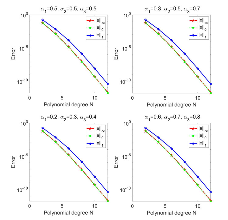
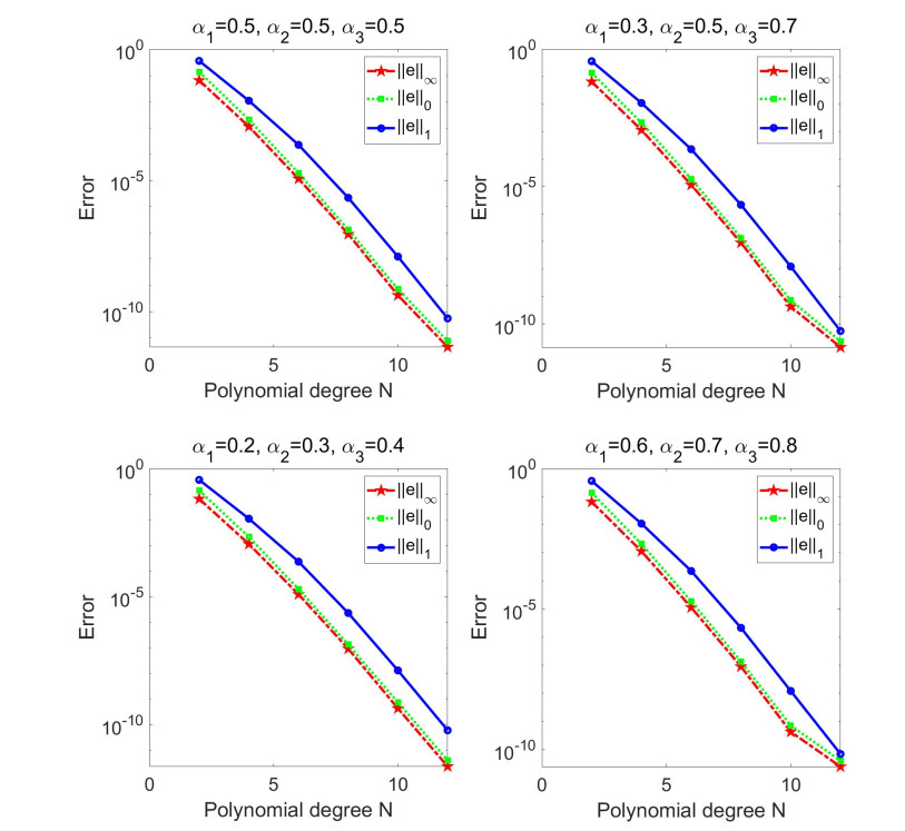
In this paper, we consider a numerical method for the multi-term Caputo-Fabrizio time-fractional diffusion equations (with orders $ \alpha_i\in(0, 1) $, $ i = 1, 2, \cdots, n $). The proposed method employs a fast finite difference scheme to approximate multi-term fractional derivatives in time, requiring only $ O(1) $ storage and $ O(N_T) $ computational complexity, where $ N_T $ denotes the total number of time steps. Then we use a Legendre spectral collocation method for spatial discretization. The stability and convergence of the scheme have been thoroughly discussed and rigorously established. We demonstrate that the proposed scheme is unconditionally stable and convergent with an order of $ O\left(\left(\Delta t\right)^{2}+N^{-m}\right) $, where $ \Delta t $, $ N $, and $ m $ represent the timestep size, polynomial degree, and regularity in the spatial variable of the exact solution, respectively. Numerical results are presented to validate the theoretical predictions.
- multi-term time-fractional diffusion equation,
- Caputo-Fabrizio derivative,
- finite difference,
- spectral approximation,
- stability,
- error estimates
Citation: Bin Fan. Efficient numerical method for multi-term time-fractional diffusion equations with Caputo-Fabrizio derivatives[J]. AIMS Mathematics, 2024, 9(3): 7293-7320. doi: 10.3934/math.2024354

Related Papers:

Abstract

In this paper, we consider a numerical method for the multi-term Caputo-Fabrizio time-fractional diffusion equations (with orders $ \alpha_i\in(0, 1) $, $ i = 1, 2, \cdots, n $). The proposed method employs a fast finite difference scheme to approximate multi-term fractional derivatives in time, requiring only $ O(1) $ storage and $ O(N_T) $ computational complexity, where $ N_T $ denotes the total number of time steps. Then we use a Legendre spectral collocation method for spatial discretization. The stability and convergence of the scheme have been thoroughly discussed and rigorously established. We demonstrate that the proposed scheme is unconditionally stable and convergent with an order of $ O\left(\left(\Delta t\right)^{2}+N^{-m}\right) $, where $ \Delta t $, $ N $, and $ m $ represent the timestep size, polynomial degree, and regularity in the spatial variable of the exact solution, respectively. Numerical results are presented to validate the theoretical predictions.

References

[1]	E. Cuesta, M. Kirane, S. A. Malik, Image structure preserving denoising using generalized fractional time integrals, Signal Process., 92 (2012), 553–563. https://doi.org/10.1016/j.sigpro.2011.09.001 doi: 10.1016/j.sigpro.2011.09.001
[2]	R. Magin, Fractional calculus in bioengineering, part 1, Crit. Rev. Biomed. Eng., 32 (2004). https://doi.org/10.1615/CritRevBiomedEng.v32.10
[3]	F. Mainardi, Fractional calculus and waves in linear viscoelasticity: An introduction to mathematical models, World Scientific: Imperial College Press, 2010. https://doi.org/10.1142/p614
[4]	R. Metzler, J. Klafter, The random walk's guide to anomalous diffusion: A fractional dynamics approach, Phys. Rep., 339 (2000), 1–77. https://doi.org/10.1016/S0370-1573(00)00070-3 doi: 10.1016/S0370-1573(00)00070-3
[5]	J. F. Zhou, X. M. Gu, Y. L. Zhao, H. Li, A fast compact difference scheme with unequal time-steps for the tempered time-fractional Black-Scholes model, Int. J. Comput. Math., 2023. https://doi.org/10.1080/00207160.2023.2254412
[6]	B. Jin, Fractional differential equations: An approach via fractional derivatives, Springer Cham Press, 2021. https://doi.org/10.1007/978-3-030-76043-4
[7]	I. Podlubny, Fractional differential equations: An introduction to fractional derivatives, fractional differential equations, to methods of their solution and some of their applications, Elsevier Science: Academic Press, 1998.
[8]	M. Caputo, M. Fabrizio, A new definition of fractional derivative without singular kernel, Progr. Fract. Differ. Appl., 1 (2015), 73–85. http://doi.org/10.12785/pfda/010201 doi: 10.12785/pfda/010201
[9]	D. Kai, G. Roberto, G. Andrea, S. Martin, Why fractional derivatives with nonsingular kernels should not be used, Fract. Calc. Appl. Anal., 23 (2020), 610–634. https://doi.org/10.1515/fca-2020-0032 doi: 10.1515/fca-2020-0032
[10]	S. Jocelyn, Fractional-order derivatives defined by continuous kernels: Are they really too restrictive?, Fractal Fract., 4 (2020), 40. https://doi.org/10.3390/fractalfract4030040 doi: 10.3390/fractalfract4030040
[11]	M. Caputo, M. Fabrizio, Applications of new time and spatial fractional derivatives with exponential kernels, Progr. Fract. Differ. Appl., 2 (2016), 1–11. https://doi.org/10.18576/pfda/020101 doi: 10.18576/pfda/020101
[12]	A. Atangana, On the new fractional derivative and application to nonlinear Fisher's reaction-diffusion equation, Appl. Math. Comput., 273 (2016), 948–956. https://doi.org/10.1016/j.amc.2015.10.021 doi: 10.1016/j.amc.2015.10.021
[13]	A. Atangana, B. S. T. Alkahtani, New model of groundwater flowing within a confine aquifer: Application of Caputo-Fabrizio derivative, Arab. J. Geosci., 9 (2016). https://doi.org/10.1007/s12517-015-2060-8
[14]	J. F. Gómez-Aguilar, M. G. López-López, V. M. Alvarado-Martínez, J. Reyes-Reyes, M. Adam-Medina, Modeling diffusive transport with a fractional derivative without singular kernel, Phys. A., 447 (2016), 467–481. https://doi.org/10.1016/j.physa.2015.12.066 doi: 10.1016/j.physa.2015.12.066
[15]	J. H. Jia, H. Wang, Analysis of asymptotic behavior of the Caputo-Fabrizio time-fractional diffusion equation, Appl. Math. Lett., 136 (2023), 108447. https://doi.org/10.1016/j.aml.2022.108447 doi: 10.1016/j.aml.2022.108447
[16]	I. A. Mirza, D. Vieru, Fundamental solutions to advection–diffusion equation with time-fractional Caputo-Fabrizio derivative, Comput. Math. Appl., 73 (2017), 1–10. https://doi.org/10.1016/j.camwa.2016.09.026 doi: 10.1016/j.camwa.2016.09.026
[17]	N. H. Tuan, Y. Zhou, Well-posedness of an initial value problem for fractional diffusion equation with Caputo-Fabrizio derivative, J. Comput. Appl. Math., 375 (2020), 112811. https://doi.org/10.1016/j.cam.2020.112811 doi: 10.1016/j.cam.2020.112811
[18]	J. D. Djida, A. Atangana, More generalized groundwater model with space-time caputo Fabrizio fractional differentiation, Numer. Meth. Part. D. E., 33 (2017), 1616–1627. https://doi.org/10.1002/num.22156 doi: 10.1002/num.22156
[19]	M. Abdulhameed, D. Vieru, R. Roslan, Modeling electro-magneto-hydrodynamic thermo-fluidic transport of biofluids with new trend of fractional derivative without singular kernel, Phys. A., 484 (2017), 233–252. https://doi.org/10.1016/j.physa.2017.05.001 doi: 10.1016/j.physa.2017.05.001
[20]	M. Al-Refai, T. Abdeljawad, Analysis of the fractional diffusion equations with fractional derivative of non-singular kernel, Adv. Differ. Equ., 2017 (2017), 315. http://dx.doi.org/10.1186/s13662-017-1356-2 doi: 10.1186/s13662-017-1356-2
[21]	N. Al-Salti, E. Karimov, S. Kerbal, Boundary-value problems for fractional heat equation involving Caputo-Fabrizio derivative, New Trends Math. Sci., 4 (2016), 79–89.
[22]	F. Liu, S. Shen, V. Anh, I. Turner, Analysis of a discrete non-Markovian random walk approximation for the time fractional diffusion equation, ANZIAM J., 46 (2004), C488–C504. https://doi.org/10.21914/anziamj.v46i0.973 doi: 10.21914/anziamj.v46i0.973
[23]	Y. M. Lin, C. J. Xu, Finite difference/spectral approximations for the time-fractional diffusion equation, J. Comput. Phys., 225 (2007), 1533–1552. https://doi.org/10.1016/j.jcp.2007.02.001 doi: 10.1016/j.jcp.2007.02.001
[24]	X. J. Li, C. J. Xu, A space-time spectral method for the time fractional diffusion equation, SIAM J. Numer. Anal., 47 (2009), 2108–2131. https://doi.org/10.1137/080718942 doi: 10.1137/080718942
[25]	J. C. Ren, Z. Z. Sun, Efficient and stable numerical methods for multi-term time fractional sub-diffusion equations, E. Asian J. Appl. Math., 4 (2014), 242–266. https://doi.org/10.4208/eajam.181113.280514a doi: 10.4208/eajam.181113.280514a
[26]	B. T. Jin, R. Lazarov, Y. K. Liu, Z. Zhou, The Galerkin finite element method for a multi-term time-fractional diffusion equation, J. Comput. Phys., 281 (2015), 825–843. https://doi.org/10.1016/j.jcp.2014.10.051 doi: 10.1016/j.jcp.2014.10.051
[27]	M. Fardi, J. Alidousti, A legendre spectral-finite difference method for Caputo–Fabrizio time-fractional distributed-order diffusion equation, Math. Sci., 16 (2022), 417–430. https://doi.org/10.1007/s40096-021-00430-4 doi: 10.1007/s40096-021-00430-4
[28]	M. Zheng, F. Liu, V. Anh, I. Turner, A high-order spectral method for the multi-term time-fractional diffusion equations, Appl. Math. Model., 40 (2016), 4970–4985. https://doi.org/10.1016/j.apm.2015.12.011 doi: 10.1016/j.apm.2015.12.011
[29]	Y. M. Zhao, Y. D. Zhang, F. Liu, I. Turner, Y. F. Tang, V. Anh, Convergence and superconvergence of a fully-discrete scheme for multi-term time fractional diffusion equations, Comput. Math. Appl., 73 (2017), 1087–1099. https://doi.org/10.1016/j.camwa.2016.05.005 doi: 10.1016/j.camwa.2016.05.005
[30]	T. Akman, B. Yıldız, D. Baleanu, New discretization of Caputo–Fabrizio derivative, Comput. Appl. Math., 37 (2018), 3307–3333. https://doi.org/10.1007/s40314-017-0514-1 doi: 10.1007/s40314-017-0514-1
[31]	F. Yu, M. H. Chen, Finite difference/spectral approximations for the two-dimensional time Caputo-Fabrizio fractional diffusion equation, arXiv, 2019. https://doi.org/10.48550/arXiv.1906.00328
[32]	J. K. Shi, M. H. Chen, A second-order accurate scheme for two-dimensional space fractional diffusion equations with time Caputo-Fabrizio fractional derivative, Appl. Numer. Math., 151 (2020), 246–262. https://doi.org/10.1016/j.apnum.2020.01.007 doi: 10.1016/j.apnum.2020.01.007
[33]	M. Taghipour, H. Aminikhah, A new compact alternating direction implicit method for solving two dimensional time fractional diffusion equation with Caputo-Fabrizio derivative, Filomat, 34 (2020), 3609–3626. https://doi.org/10.2298/FIL2011609T doi: 10.2298/FIL2011609T
[34]	S. D. Jiang, J. W. Zhang, Q. Zhang, Z. M. Zhang, Fast evaluation of the Caputo fractional derivative and its applications to fractional diffusion equations, Commun. Comput. Phys., 21 (2017), 650–678. https://doi.org/10.4208/cicp.OA-2016-0136 doi: 10.4208/cicp.OA-2016-0136
[35]	M. Li, X. M. Gu, C. M. Huang, M. F. Fei, G. Y. Zhang, A fast linearized conservative finite element method for the strongly coupled nonlinear fractional Schrödinger equations, J. Comput. Phys., 358 (2018), 256–282. https://doi.org/10.1016/j.jcp.2017.12.044 doi: 10.1016/j.jcp.2017.12.044
[36]	F. H. Zeng, I. Turner, K. Burrage, A stable fast time-stepping method for fractional integral and derivative operators, J. Sci. Comput., 77 (2018), 283–307. https://doi.org/10.1007/s10915-018-0707-9 doi: 10.1007/s10915-018-0707-9
[37]	H. Y. Zhu, C. J. Xu, A fast high order method for the time-fractional diffusion equation, SIAM J. Numer. Anal., 57 (2019), 2829–2849. https://doi.org/10.1137/18M1231225 doi: 10.1137/18M1231225
[38]	H. Liu, A. J. Cheng, H. J. Yan, Z. G. Liu, H. Wang, A fast compact finite difference method for quasilinear time fractional parabolic equation without singular kernel, Int. J. Comput. Math., 96 (2019), 1444–1460. https://doi.org/10.1080/00207160.2018.1501479 doi: 10.1080/00207160.2018.1501479
[39]	Y. Liu, E. N. Fan, B. L. Yin, H. Li, Fast algorithm based on the novel approximation formula for the Caputo-Fabrizio fractional derivative, AIMS Math., 5 (2020), 1729–1744. https://doi.org/10.3934/math.2020117 doi: 10.3934/math.2020117
[40]	X. M. Gu, S. L. Wu, A parallel-in-time iterative algorithm for Volterra partial integro-differential problems with weakly singular kernel, J. Comput. Phys., 417 (2020), 109576. https://doi.org/10.1016/j.jcp.2020.109576 doi: 10.1016/j.jcp.2020.109576
[41]	C. Bernardi, Y. Maday, Approximations spectrales de problemes aux limites elliptiques, Berlin: Springer Press, 142 (1992).
[42]	A. Quarteroni, A. Valli, Numerical approximation of partial differential equations, Springer Science & Business Media, 2008. https://doi.org/10.1007/978-3-540-85268-1

Reader Comments

Your name:*

Email:*
© 2024 the Author(s), licensee AIMS Press. This is an open access article distributed under the terms of the Creative Commons Attribution License (http://creativecommons.org/licenses/by/4.0)