As a powerful tool for describing and studying the properties of networks, the graph spectrum analyses and calculations have attracted substantial attention from the scientific community. Let $ C_{n} $ represent linear crossed phenylenes. Based on the Laplacian (normalized Laplacian, resp.) polynomial of $ C_{n} $, we first investigated the Laplacian (normalized Laplacian, resp) spectrum of $ C_{n} $ in this paper. Furthermore, the Kirchhoff index, multiplicative degree-Kirchhoff, index and complexity of $ C_{n} $ were obtained through the relationship between the roots and the coefficients of the characteristic polynomials. Finally, it was found that the Kirchhoff index and multiplicative degree-Kirchhoff index of $ C_{n} $ were approximately one quarter of their Wiener index and Gutman index, respectively.
Citation: Zhi-Yu Shi, Jia-Bao Liu. Topological indices of linear crossed phenylenes with respect to their Laplacian and normalized Laplacian spectrum[J]. AIMS Mathematics, 2024, 9(3): 5431-5450. doi: 10.3934/math.2024262
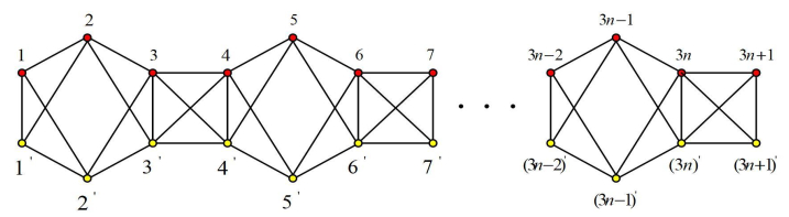
As a powerful tool for describing and studying the properties of networks, the graph spectrum analyses and calculations have attracted substantial attention from the scientific community. Let $ C_{n} $ represent linear crossed phenylenes. Based on the Laplacian (normalized Laplacian, resp.) polynomial of $ C_{n} $, we first investigated the Laplacian (normalized Laplacian, resp) spectrum of $ C_{n} $ in this paper. Furthermore, the Kirchhoff index, multiplicative degree-Kirchhoff, index and complexity of $ C_{n} $ were obtained through the relationship between the roots and the coefficients of the characteristic polynomials. Finally, it was found that the Kirchhoff index and multiplicative degree-Kirchhoff index of $ C_{n} $ were approximately one quarter of their Wiener index and Gutman index, respectively.

| [1] |
J. Chen, A. B. Le, Q. Wang, L. Xi, A small-world and scale-free network generated by Sierpinski Pentagon, Physica A, 449 (2016), 126–135. https://doi.org/10.1016/j.physa.2015.12.089 doi: 10.1016/j.physa.2015.12.089

|
| [2] |
W. Sun, M. Sun, J. Guan, Q. Jia, Robustness of coherence in noisy scale-free networks and applications to identification of influential spreaders, IEEE T. Circuits-Ⅱ, 67 (2019), 1274–1278. https://doi.org/10.1109/TCSII.2019.2929139 doi: 10.1109/TCSII.2019.2929139
|
| [3] |
W. Sun, Q. Ding, J. Zhang, F. Chen, Coherence in a family of tree networks with an application of Laplacian spectrum, Chaos, 24 (2014), 043112. https://doi.org/10.1063/1.4897568 doi: 10.1063/1.4897568
|
| [4] |
X. Qi, E. Fuller, R. Luo, G. Guo, C. Zhang, Laplacian energy of digraphs and a minimum Laplacian energy algorithm, Int. J. Found. Comput. Sci., 26 (2015), 367–380. https://doi.org/10.1142/S0129054115500203 doi: 10.1142/S0129054115500203
|
| [5] |
Y. J. Yang, H. P. Zhang, Kirchhoff index of linear hexagonal chains, Int. J. Quantum Chem., 108 (2008), 503–512. https://doi.org/10.1002/qua.21537 doi: 10.1002/qua.21537
|
| [6] |
J. Huang, S. C. Li, L. Sun, The normalized Laplacians degree-Kirchhoff index and the spanning trees of linear hexagonal chains, Discrete Appl. Math., 207 (2016), 67–79. https://doi.org/10.1016/j.dam.2016.02.019 doi: 10.1016/j.dam.2016.02.019
|
| [7] | Y. J. Peng, S. C. Li, On the kirchhoff index and the number of spanning trees of linear phenylenes, Match Communications in Mathematical and in Computer Chemistry, 77 (2017), 765–780. |
| [8] |
Z. X. Zhu, J. B. Liu, The normalized Laplacian, degree-Kirchhoff index and the spanning tree numbers of generalized phenylenes, Discrete Appl. Math., 254 (2019), 256–267. https://doi.org/10.1016/j.dam.2018.06.026 doi: 10.1016/j.dam.2018.06.026
|
| [9] |
Y. Pan, J. Li, Kirchhoff index, multiplicative degree-Kirchhoff index and spanning trees of the linear crossed hexagonal chains, Int. J. Quantum Chem., 118 (2018), e25787. https://doi.org/10.1002/qua.25787 doi: 10.1002/qua.25787
|
| [10] |
D. Zhao, Y. Zhao, Z. Wang, X. Li, K. Zhou, Kirchhoff index and degree Kirchhoff index of Tetrahedrane-derived compounds, Symmetry, 15 (2023), 1122. https://doi.org/10.3390/sym15051122 doi: 10.3390/sym15051122
|
| [11] | J. Wang, L. Liu, H. Zhang, On the Laplacian spectra and the Kirchhoff indices of two types of networks, Optimization, (2023). https://doi.org/10.1080/02331934.2023.2268631 |
| [12] |
X. Geng, P. Wang, L. Lei, S. Wang, On the Kirchhoff indices and the number of spanning trees of M$\ddot{o}$bius phenylenes chain and Cylinder phenylenes chain, Polycycl. Aromat. Comp., 41 (2021), 1681–1693. https://doi.org/10.1080/10406638.2019.1693405 doi: 10.1080/10406638.2019.1693405
|
| [13] |
X. Ma, H. Bian, The normalized Laplacians, degree-Kirchhoff index and the spanning trees of hexagonal M$\ddot{o}$bius graphs, Appl. Math. Comput., 355 (2019), 33–46. https://doi.org/10.1016/j.amc.2019.02.052 doi: 10.1016/j.amc.2019.02.052
|
| [14] |
J. Huang, S. C. Li, X. Li, The normalized Laplacian, degree-Kirchhoff index and spanning trees of the linear polyomino chains, Appl. Math. Comput., 289 (2016), 324–334. https://doi.org/10.1016/j.amc.2016.05.024 doi: 10.1016/j.amc.2016.05.024
|
| [15] | F. R. K. Chung, Spectral Graph Theory, American Mathematical Society Providence, RI, 1997. |
| [16] |
H. Wiener, Structural determination of paraffin boiling points, J. Am. Chem. Soc., 69 (1947), 17–20. https://doi.org/10.1021/ja01193a005 doi: 10.1021/ja01193a005
|
| [17] | A. Dobrynin, Branchings in trees and the calculation of the Wiener index of a tree, Match Communications in Mathematical and in Computer Chemistry, 41 (2000), 119–134. |
| [18] |
I. Gutman, Selected properties of the Schultz molecular topological index, Journal of Chemical Information and Computer Sciences, 34 (1994), 1087–1089. https://doi.org/10.1021/ci00021a009 doi: 10.1021/ci00021a009
|
| [19] |
D. J. Klein, M. Randić, Resistance distances, J. Math. Chem., 12 (1993), 81–95. https://doi.org/10.1007/BF01164627 doi: 10.1007/BF01164627
|
| [20] | D. J. Klein, Resistance-distance sum rules, Croat. Chem. Acta, 75 (2002), 633–649. https://hrcak.srce.hr/127542 |
| [21] |
D. J. Klein, O. Ivanciuc, Graph cyclicity, excess conductance, and resistance deficit, J. Math. Chem., 30 (2001), 271–287. https://doi.org/10.1023/A:1015119609980 doi: 10.1023/A:1015119609980
|
| [22] |
H. Y. Chen, F. J. Zhang, Resistance distance and the normalized Laplacian spectrum, Discrete Appl. Math., 155 (2007), 654–661. https://doi.org/10.1016/j.dam.2006.09.008 doi: 10.1016/j.dam.2006.09.008
|
| [23] |
I. Gutman, B. Mohar, The quasi-Wiener and the Kirchhoff indices coincide, J. Chem. Inf. Model., 36 (1996), 982–985. https://doi.org/10.1021/ci960007t doi: 10.1021/ci960007t
|
| [24] |
Y. L. Yang, T. Y. Yu, Graph theory of viscoelasticities for polymers with starshaped, multiple-ring and cyclic multiple-ring molecules, Macromol. Chem. Phys., 186 (1985), 609–631. https://doi.org/10.1002/macp.1985.021860315 doi: 10.1002/macp.1985.021860315
|
Figures(1) / Tables(3)

Zhi-Yu Shi, Jia-Bao Liu. Topological indices of linear crossed phenylenes with respect to their Laplacian and normalized Laplacian spectrum[J]. AIMS Mathematics, 2024, 9(3): 5431-5450. doi: 10.3934/math.2024262


 DownLoad: