The traveling wave solution and dynamics analysis of the fractional order generalized Pochhammer–Chree equation

Chunyan Liu; Chunyan Liu

doi:10.3934/math.20241619

AIMS Mathematics

2024, Volume 9, Issue 12: 33956-33972. doi: 10.3934/math.20241619

Previous Article Next Article

Research article

The traveling wave solution and dynamics analysis of the fractional order generalized Pochhammer–Chree equation

Chunyan Liu ^,

College of Computer Science, Chengdu University, Chengdu 610106, China

Received: 31 July 2024 Revised: 10 November 2024 Accepted: 26 November 2024 Published: 02 December 2024
MSC : 34L30, 35B20, 35C05, 35C07

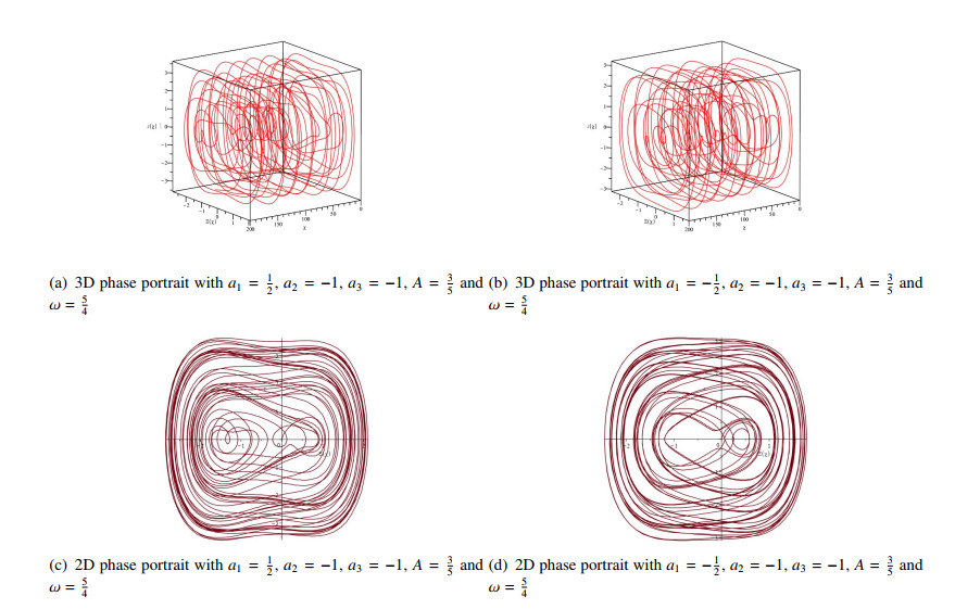
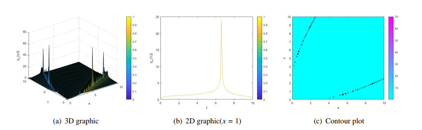
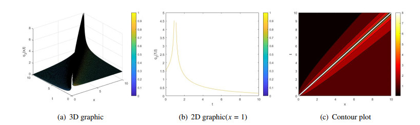
This article studies the phase portraits, chaotic patterns, and traveling wave solutions of the fractional order generalized Pochhammer–Chree equation. First, the fractional order generalized Pochhammer–Chree equation is transformed into an ordinary differential equation. Second, the dynamic behavior is analyzed using the planar dynamical system, and some three-dimensional and two-dimensional phase portraits are drawn using Maple software to reflect its chaotic behaviors. Finally, many solutions were constructed using the polynomial complete discriminant system method, including rational, trigonometric, hyperbolic, Jacobian elliptic function, and implicit function solutions. Two-dimensional graphics, three-dimensional graphics, and contour plots of some solutions are drawn.
- traveling wave solution,
- dynamics analysis,
- fractional,
- Pochhammer–Chree equation
Citation: Chunyan Liu. The traveling wave solution and dynamics analysis of the fractional order generalized Pochhammer–Chree equation[J]. AIMS Mathematics, 2024, 9(12): 33956-33972. doi: 10.3934/math.20241619

Related Papers:

Abstract

This article studies the phase portraits, chaotic patterns, and traveling wave solutions of the fractional order generalized Pochhammer–Chree equation. First, the fractional order generalized Pochhammer–Chree equation is transformed into an ordinary differential equation. Second, the dynamic behavior is analyzed using the planar dynamical system, and some three-dimensional and two-dimensional phase portraits are drawn using Maple software to reflect its chaotic behaviors. Finally, many solutions were constructed using the polynomial complete discriminant system method, including rational, trigonometric, hyperbolic, Jacobian elliptic function, and implicit function solutions. Two-dimensional graphics, three-dimensional graphics, and contour plots of some solutions are drawn.

References

[1]	S. Behera, J. P. S. Virdi, Some more solitary traveling wave solutions of nonlinear evolution equations, Interdisciplinary J. Discontinuity, Nonlinearity, Complexity, 12 (2023), 75–85. https://doi.org/10.5890/dnc.2023.03.006 doi: 10.5890/dnc.2023.03.006
[2]	S Behera, N. H. Aljahdaly, Nonlinear evolution equations and their traveling wave solutions in fluid media by modified analytical method, Pramana-J. Phys., 97 (2023), 130. https://doi.org/10.1007/s12043-023-02602-4 doi: 10.1007/s12043-023-02602-4
[3]	S. Behera, Analysis of traveling wave solutions of two space-time nonlinear fractional differential equations by the first-integral method, Mod. Phys. Lett. B, 38 (2024), 2350247. https://doi.org/10.1142/S0217984923502470 doi: 10.1142/S0217984923502470
[4]	S. Zhao, Chaos analysis and traveling wave solutions for fractional (3+1)-dimensional Wazwaz Kaur Boussinesq equation with beta derivative, Sci. Rep., 14 (2024), 23034. https://doi.org/10.1038/s41598-024-74606-y doi: 10.1038/s41598-024-74606-y
[5]	J. Dahne, Highest cusped waves for the fractional KdV equations, J. Differ. Equations, 401 (2024), 550–670. https://doi.org/10.1016/j.jde.2024.05.016 doi: 10.1016/j.jde.2024.05.016
[6]	M. Odabasi, Traveling wave solutions of conformable time-fractional Zakharov–Kuznetsov and Zoomeron equations, Chinese J. Phys., 64 (2020), 194–202. https://doi.org/10.1016/j.cjph.2019.11.003 doi: 10.1016/j.cjph.2019.11.003
[7]	B. Datsko, V. Gafiychuk, I. Podlubny, Solitary travelling auto-waves in fractional reaction–diffusion systems, Commun. Nonlinear Sci. Numer. Simul., 23 (2015), 378–387. https://doi.org/10.1016/j.cnsns.2014.10.028 doi: 10.1016/j.cnsns.2014.10.028
[8]	E. Fendzi Donfack, J. P. Nguenang, L. Nana, On the traveling waves in nonlinear electrical transmission lines with intrinsic fractional-order using discrete tanh method, Chaos, Soliton. Fract., 131 (2020), 109486. https://doi.org/10.1016/j.chaos.2019.109486 doi: 10.1016/j.chaos.2019.109486
[9]	A. Das, N. Ghosh, K. Ansari, Bifurcation and exact traveling wave solutions for dual power Zakharov–Kuznetsov–Burgers equation with fractional temporal evolution, Comput. Math. Appl., 75 (2018), 59–69. https://doi.org/10.1016/j.camwa.2017.08.043 doi: 10.1016/j.camwa.2017.08.043
[10]	K. Wang, Exact travelling wave solution for the local fractional Camassa-Holm-Kadomtsev-Petviashvili equation, Alex. Eng. J., 63 (2023), 371–376. https://doi.org/10.1016/j.aej.2022.08.011 doi: 10.1016/j.aej.2022.08.011
[11]	M. Eslami, Exact traveling wave solutions to the fractional coupled nonlinear Schrodinger equations, Appl. Math. Comput., 285 (2016), 141–148. https://doi.org/10.1016/j.amc.2016.03.032 doi: 10.1016/j.amc.2016.03.032
[12]	T. Islam, M. A. Akbar, A. K. Azad, Traveling wave solutions to some nonlinear fractional partial differential equations through the rational ($G'/G$)-expansion method, J. Ocean Eng. Sci., 3 (2018), 76–81. https://doi.org/10.1016/j.joes.2017.12.003 doi: 10.1016/j.joes.2017.12.003
[13]	M. Mamunur Roshid, M. Uddin, G. Mostafa, Dynamical structure of optical soliton solutions for M-fractional paraxial wave equation by using unified technique, Results Phys., 51 (2023), 106632. https://doi.org/10.1016/j.rinp.2023.106632 doi: 10.1016/j.rinp.2023.106632
[14]	C. S. Liu, Applications of complete discrimination system for polynomial for classifications of traveling wave solutions to nonlinear differential equations, Comput. Phys. Commun., 181 (2010), 317–324. https://doi.org/10.1016/j.cpc.2009.10.006 doi: 10.1016/j.cpc.2009.10.006
[15]	J. Li, Z. Liu, Smooth and non-smooth traveling waves in a nonlinearly dispersive equation, Appl. Math. Model., 25 (2020), 41–56. https://doi.org/10.1016/S0307-904X(00)00031-7 doi: 10.1016/S0307-904X(00)00031-7
[16]	C. Liu, The chaotic behavior and traveling wave solutions of the conformable extended Korteweg-de-Vries model, Open Phys., 22 (2024), 20240069. https://doi.org/10.1515/phys-2024-0069 doi: 10.1515/phys-2024-0069
[17]	Z. Li, T. Han, Bifurcation and exact solutions for the (2+1)-dimensional conformable time-fractional Zoomeron equation, Adv. Differ. Equ., 2020 (2020), 656. https://doi.org/10.1186/s13662-020-03119-5 doi: 10.1186/s13662-020-03119-5
[18]	A. Zulfiqar, J. Ahmad, Q. M. Ul-Hassan, Analysis of some new wave solutions of fractional order generalized Pochhammer-chree equation using exp-function method, Opt. Quant. Electron., 54 (2022), 735. https://doi.org/10.1007/s11082-022-04141-5 doi: 10.1007/s11082-022-04141-5
[19]	S. Tarla, K. K. Ali, H. Günerhan, Optical soliton solutions of generalized Pochammer Chree equation, Opt. Quant. Electron., 56 (2024), 899. https://doi.org/10.1007/s11082-024-06711-1 doi: 10.1007/s11082-024-06711-1
[20]	N. Abbas, A. Hussain, A. Khan, T. Abdeljawad, Bifurcation analysis, quasi-periodic and chaotic behavior of generalized Pochhammer-Chree equation, Ain Shams Eng. J., 15 (2024), 102827. https://doi.org/10.1016/j.asej.2024.102827 doi: 10.1016/j.asej.2024.102827
[21]	A. K. Hussain, M. Y. Usman, F. Zaman, S. M. Eldin, Double reductions and traveling wave structures of the generalized Pochhammer-Chree equation, Partial Differ. Equ. Appl. Math., 7 (2023), 100521. https://doi.org/10.1016/j.padiff.2023.100521 doi: 10.1016/j.padiff.2023.100521
[22]	A. EL Achab, On the integrability of the generalized Pochhammer-Chree (PC) equations, Phys. A: Stat. Mech. Appl., 545 (2020), 123576. https://doi.org/10.1016/j.physa.2019.123576 doi: 10.1016/j.physa.2019.123576
[23]	J. Li, L. Zhang, Bifurcations of traveling wave solutions in generalized Pochhammer-Chree equation, Chaos, Soliton. Fract., 14 (2002), 581–593. https://doi.org/10.1016/S0960-0779(01)00248-X doi: 10.1016/S0960-0779(01)00248-X
[24]	Y. Cheng, Classification of traveling wave solutions to the Vakhnenko equations, Comput. Math. Appl., 62 (2011), 3987–3996. https://doi.org/10.1016/j.camwa.2011.09.060 doi: 10.1016/j.camwa.2011.09.060
[25]	Y. Kai, S. Chen, B. Zheng, K. Zhang, N. Yang, W. Xu, Qualitative and quantitative analysis of nonlinear dynamics by the complete discrimination system for polynomial method, Chaos, Soliton. Fract., 141 (2020), 110314. https://doi.org/10.1016/j.chaos.2020.110314 doi: 10.1016/j.chaos.2020.110314

Reader Comments

Your name:*

Email:*
© 2024 the Author(s), licensee AIMS Press. This is an open access article distributed under the terms of the Creative Commons Attribution License (http://creativecommons.org/licenses/by/4.0)