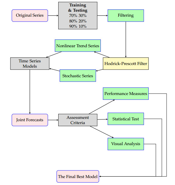
Traders and investors find predicting stock market values an intriguing subject to study in stock exchange markets. Accurate projections lead to high financial revenues and protect investors from market risks. This research proposes a unique filtering-combination approach to increase forecast accuracy. The first step is to filter the original series of stock market prices into two new series, consisting of a nonlinear trend series in the long run and a stochastic component of a series, using the Hodrick-Prescott filter. Next, all possible filtered combination models are considered to get the forecasts of each filtered series with linear and nonlinear time series forecasting models. Then, the forecast results of each filtered series are combined to extract the final forecasts. The proposed filtering-combination technique is applied to Pakistan's daily stock market price index data from January 2, 2013 to February 17, 2023. To assess the proposed forecasting methodology's performance in terms of model consistency, efficiency and accuracy, we analyze models in different data set ratios and calculate four mean errors, correlation coefficients and directional mean accuracy. Last, the authors recommend testing the proposed filtering-combination approach for additional complicated financial time series data in the future to achieve highly accurate, efficient and consistent forecasts.
Citation: Hasnain Iftikhar, Murad Khan, Josué E. Turpo-Chaparro, Paulo Canas Rodrigues, Javier Linkolk López-Gonzales. Forecasting stock prices using a novel filtering-combination technique: Application to the Pakistan stock exchange[J]. AIMS Mathematics, 2024, 9(2): 3264-3288. doi: 10.3934/math.2024159
Traders and investors find predicting stock market values an intriguing subject to study in stock exchange markets. Accurate projections lead to high financial revenues and protect investors from market risks. This research proposes a unique filtering-combination approach to increase forecast accuracy. The first step is to filter the original series of stock market prices into two new series, consisting of a nonlinear trend series in the long run and a stochastic component of a series, using the Hodrick-Prescott filter. Next, all possible filtered combination models are considered to get the forecasts of each filtered series with linear and nonlinear time series forecasting models. Then, the forecast results of each filtered series are combined to extract the final forecasts. The proposed filtering-combination technique is applied to Pakistan's daily stock market price index data from January 2, 2013 to February 17, 2023. To assess the proposed forecasting methodology's performance in terms of model consistency, efficiency and accuracy, we analyze models in different data set ratios and calculate four mean errors, correlation coefficients and directional mean accuracy. Last, the authors recommend testing the proposed filtering-combination approach for additional complicated financial time series data in the future to achieve highly accurate, efficient and consistent forecasts.

| [1] | L. O. Petram, The world's first stock exchange: How the Amsterdam market for Dutch East India Company shares became a modern securities market, Doctoral dissertation, Universiteit van Amsterdam, 2011, 1602–1700. |
| [2] |
L. A. Castillo, M. J. Orraca, G. S. Molina, The global component of headline and core inflation in emerging market economies and its ability to improve forecasting performance, Econ. Model., 120 (2023), 106121. https://doi.org/10.1016/j.econmod.2022.106121 doi: 10.1016/j.econmod.2022.106121

|
| [3] |
C. He, K. Huang, J. Lin, T. Wang, Z. Zhang, Explain systemic risk of commodity futures market by dynamic network, Int. Rev. Financ. Anal., 88 (2023), 102658. https://doi.org/10.1016/j.irfa.2023.102658 doi: 10.1016/j.irfa.2023.102658
|
| [4] |
I. K. Nti, A. F. Adekoya, B. A. Weyori, A systematic review of fundamental and technical analysis of stock market predictions, Artif. Intell. Rev., 53 (2020), 3007–3057. https://doi.org/10.1007/s10462-019-09754-z doi: 10.1007/s10462-019-09754-z
|
| [5] |
Z. Li, X. Zhou, S. Huang, Managing skill certification in online outsourcing platforms: A perspective of buyer-determined reverse auctions, Int. J. Prod. Econ., 238 (2021), 108166. https://doi.org/10.1016/j.ijpe.2021.108166 doi: 10.1016/j.ijpe.2021.108166
|
| [6] |
E. Catullo, M. Gallegati, A. Russo, Forecasting in a complex environment: Machine learning sales expectations in a stock flow consistent agent-based simulation model, J. Econ. Dyn. Control, 139 (2022), 104405. https://doi.org/10.1016/j.jedc.2022.104405 doi: 10.1016/j.jedc.2022.104405
|
| [7] |
A. Bucci, G. Palomba, E. Rossi, The role of uncertainty in forecasting volatility comovements across stock markets, Econ. Modell., 125 (2023), 106309. https://doi.org/10.1016/j.econmod.2023.106309 doi: 10.1016/j.econmod.2023.106309
|
| [8] |
M. M. Kumbure, C. Lohrmann, P. Luukka, J. Porras, Machine learning techniques and data for stock market forecasting: A literature review, Expert Syst. Appl., 2022, 116659. https://doi.org/10.1016/j.eswa.2022.116659 doi: 10.1016/j.eswa.2022.116659
|
| [9] |
H. Iftikhar, J. E. T. Chaparro, P. C. Rodrigues, J. L. López-Gonzales, Forecasting Day-Ahead electricity prices for the Italian electricity market using a new decomposition-combination technique, Energies, 16 (2023), 6669. https://doi.org/10.3390/en16186669 doi: 10.3390/en16186669
|
| [10] |
N. C. Bustinza, H. Iftikhar, M. Belmonte, R. J. C. Torres, A. R. H. De La Cruz, J. L. López-Gonzales, Short-term forecasting of Ozone concentration in metropolitan Lima using hybrid combinations of time series models, Appl. Sci., 13 (2023), 10514. https://doi.org/10.3390/app131810514 doi: 10.3390/app131810514
|
| [11] |
X. Li, Y. Sun, Stock intelligent investment strategy based on support vector machine parameter optimization algorithm, Neural Comput. Appl., 32 (2020), 1765–1775. https://doi.org/10.1007/s00521-019-04566-2 doi: 10.1007/s00521-019-04566-2
|
| [12] |
P. Mondal, L. Shit, S. Goswami, Study of effectiveness of time series modeling (ARIMA) in forecasting stock prices, Int. J. Comput. Sci. Eng. Appl., 4 (2014), 13. https://doi.org/10.5121/ijcsea.2014.4202 doi: 10.5121/ijcsea.2014.4202
|
| [13] |
B. Wang, H. Huang, X. Wang, A novel text mining approach to financial time series forecasting, Neurocomputing, 83 (2012), 136–145. https://doi.org/10.1016/j.neucom.2011.12.013 doi: 10.1016/j.neucom.2011.12.013
|
| [14] |
M. Ghani, Q. Guo, F. Ma, T. Li, Forecasting Pakistan stock market volatility: Evidence from economic variables and the uncertainty index, Int. Rev. Econ. Financ., 80 (2022), 1180–1189. https://doi.org/10.1016/j.iref.2022.04.003 doi: 10.1016/j.iref.2022.04.003
|
| [15] |
D. Kumar, P. K. Sarangi, R. Verma, A systematic review of stock market prediction using machine learning and statistical techniques, Materials Today Proc., 49 (2022), 3187–3191. https://doi.org/10.1016/j.matpr.2020.11.399 doi: 10.1016/j.matpr.2020.11.399
|
| [16] |
S. Raubitzek, T. Neubauer, An exploratory study on the complexity and machine learning predictability of stock market data, Entropy, 24 (2022), 332. https://doi.org/10.3390/e24030332 doi: 10.3390/e24030332
|
| [17] |
X. Li, Y. Sun, Application of RBF neural network optimal segmentation algorithm in credit rating, Neural Comput. Appl., 33 (2021), 8227–8235. https://doi.org/10.1007/s00521-020-04958-9 doi: 10.1007/s00521-020-04958-9
|
| [18] |
H. Dichtl, W. Drobetz, T. Otto, Forecasting stock market crashes via machine learning, J. Financ. Stabil., 65 (2023), 101099. https://doi.org/10.1016/j.jfs.2022.101099 doi: 10.1016/j.jfs.2022.101099
|
| [19] | J. Kamruzzaman, R. A. Sarker, ANN-based forecasting of foreign currency exchange rates, Neural Inform. Process.-Lett. Rev., 3 (2004), 49–58. |
| [20] |
H. Iftikhar, A. Zafar, J. E. T. Chaparro, P. C. Rodrigues, J. L. López-Gonzales, Forecasting Day-Ahead Brent crude oil prices using hybrid combinations of time series models, Mathematics, 11 (2023), 3548. https://doi.org/10.3390/math11163548 doi: 10.3390/math11163548
|
| [21] |
C. Ma, D. Wen, G. J. Wang, Y. Jiang, Further mining the predictability of moving averages: Evidence from the US stock market, Int. Rev. Financ., 19 (2019), 413–433. https://doi.org/10.1111/irfi.12166 doi: 10.1111/irfi.12166
|
| [22] |
Z. Jiang, C. Xu, Disrupting the technology innovation efficiency of manufacturing enterprises through digital technology promotion: An evidence of 5G technology construction in China, IEEE T. Eng. Manage., 2023. https://doi.org/10.1109/TEM.2023.3261940 doi: 10.1109/TEM.2023.3261940
|
| [23] |
L. Lin, Y. Jiang, H. Xiao, Z. Zhou, Crude oil price forecasting based on a novel hybrid long memory GARCH-M and wavelet analysis model, Phys. A, 543 (2020), 123532. https://doi.org/10.1016/j.physa.2019.123532 doi: 10.1016/j.physa.2019.123532
|
| [24] |
Z. Zhou, Y. Jiang, Y. Liu, L. Lin, Q. Liu, Does international oil volatility have directional predictability for stock returns? Evidence from BRICS countries based on cross-quantilogram analysis, Econ. Modell., 80 (2019), 352–382. https://doi.org/10.1016/j.econmod.2018.11.021 doi: 10.1016/j.econmod.2018.11.021
|
| [25] |
C. H. Cheng, M. C. Tsai, C. Chang, A time series model based on deep learning and integrated indicator selection method for forecasting stock prices and evaluating trading profits, Systems, 10 (2022), 243. https://doi.org/10.3390/systems10060243 doi: 10.3390/systems10060243
|
| [26] |
Y. Han, J. Kim, D. Enke, A machine learning trading system for the stock market based on N-period Min-Max labeling using XGBoost, Expert Syst. Appl., 211 (2023), 118581. https://doi.org/10.1016/j.eswa.2022.118581 doi: 10.1016/j.eswa.2022.118581
|
| [27] |
H. Iftikhar, N. Bibi, P. C. Rodrigues, J. L. López-Gonzales, Multiple novel decomposition techniques for time series forecasting: Application to monthly forecasting of electricity consumption in Pakistan, Energies, 2023 (2023), 2579. https://doi.org/10.3390/en16062579 doi: 10.3390/en16062579
|
| [28] |
H. Iftikhar, M. Daniyal, M. Qureshi, K. Tawaiah, R. K. Ansah, J. K. Afriyie, A hybrid forecasting technique for infection and death from the mpox virus, Digit. Health, 9 (2023). https://doi.org/10.1177/20552076231204748 doi: 10.1177/20552076231204748
|
| [29] |
H. Iftikhar, J. E. T. Chaparro, P. C. Rodrigues, J. L. López-Gonzales, Day-Ahead electricity demand forecasting using a novel decomposition combination method, Energies, 16 (2023), 6675. https://doi.org/10.3390/en16186675 doi: 10.3390/en16186675
|
| [30] |
H. Iftikhar, M. Khan, M. S. Khan, M. Khan, Short-term forecasting of Monkeypox cases using a novel filtering and combining technique, Diagnostics, 13 (2023), 1923. https://doi.org/10.3390/diagnostics13111923 doi: 10.3390/diagnostics13111923
|
| [31] |
Q. M. Ilyas, K. Iqbal, S. Ijaz, A. Mehmood, S. Bhatia, A hybrid model to predict stock closing price using novel features and a fully modified Hodrick-Prescott filter, Electronics, 11 (2022), 3588. https://doi.org/10.3390/electronics11213588 doi: 10.3390/electronics11213588
|
| [32] |
I. Daubechies, J. Lu, H. T. Wu, Synchrosqueezed wavelet transforms: An empirical mode decomposition-like tool, Appl. Comput. Harmon. A., 30 (2011), 243–261. https://doi.org/10.1016/j.acha.2010.08.002 doi: 10.1016/j.acha.2010.08.002
|
| [33] |
Z. Zhou, L. Lin, S. Li, International stock market contagion: A CEEMDAN wavelet analysis, Econ. Model., 72 (2018), 333–352. https://doi.org/10.1016/j.econmod.2018.02.010 doi: 10.1016/j.econmod.2018.02.010
|
| [34] |
M. Ali, D. M. Khan, H. M. Alshanbari, A. A. A. H. El-Bagoury, Prediction of complex stock market data using an improved hybrid EMD-LSTM model, Appl. Sci., 13 (2023), 1429. https://doi.org/10.3390/app13031429 doi: 10.3390/app13031429
|
| [35] |
I. Shah, H. Iftikhar, S. Ali, D. Wang, Short-term electricity demand forecasting using components estimation technique, Energies, 12 (2019), 2532. https://doi.org/10.3390/en12132532 doi: 10.3390/en12132532
|
| [36] | H. Iftikhar, Modeling and forecasting complex time series: A case of electricity demand, M. Phil, thesis, Quaidi-Azam University, Islamabad, Pakistan, 2018, 1–94. |
| [37] |
I. Shah, H. Iftikhar, S. Ali, Modeling and forecasting electricity demand and prices: A comparison of alternative approaches, J. Math., 2022 (2022), 3581037. https://doi.org/10.1155/2022/3581037 doi: 10.1155/2022/3581037
|
| [38] |
F. X. Diebold, R. S. Mariano, Comparing predictive accuracy, J. Bus. Econ. Stat., 20 (2002), 134–144. https://doi.org/10.1198/073500102753410444 doi: 10.1198/073500102753410444
|
| [39] |
I. Shah, H. Iftikhar, S. Ali, Modeling and forecasting medium-term electricity consumption using component estimation technique, Forecasting, 2 (2020), 163–179. https://doi.org/10.3390/forecast2020009 doi: 10.3390/forecast2020009
|
| [40] |
H. Iftikhar, M. Khan, Z. Khan, F. Khan, H. M. Alshanbari, Z. Ahmad, A comparative analysis of machine learning models: A case study in predicting chronic kidney disease, Sustainability, 15 (2023), 2754. https://doi.org/10.3390/su15032754 doi: 10.3390/su15032754
|
| [41] |
H. M. Alshanbari, H. Iftikhar, F. Khan, M. Rind, Z. Ahmad, A. A. A. H. El-Bagoury, On the implementation of the artificial neural network approach for forecasting different healthcare events, Diagnostics, 7 (2023), 1310. https://doi.org/10.3390/diagnostics13071310 doi: 10.3390/diagnostics13071310
|
| [42] |
D. A. Dickey, W. A. Fuller, Distribution of the estimators for autoregressive time series with a unit root, J. Am. Stat. Assoc., 74 (1979), 427–431. https://doi.org/10.1080/01621459.1979.10482531 doi: 10.1080/01621459.1979.10482531
|
| [43] |
T. Teraesvirta, C. F. Lin, C. W. J. Granger, Power of the neural network linearity test, J. Time Ser. Anal., 14 (1993), 209–220. https://doi.org/10.1111/j.1467-9892.1993.tb00139.x doi: 10.1111/j.1467-9892.1993.tb00139.x
|
| [44] | P. J. Brockwell, R. A. Davis, Introduction to time series and forecasting, Berlin/Heidelberg: Springer, 2016. |
| [45] |
Q. Gu, S. Li, Z. Liao, Solving nonlinear equation systems based on evolutionary multitasking with neighborhood-based speciation differential evolution, Expert Syst. Appl., 238 (2024), 122025. https://doi.org/10.1016/j.eswa.2023.122025 doi: 10.1016/j.eswa.2023.122025
|
| [46] |
M. Dritsaki, C. Dritsaki, Comparison of HP filter and the Hamilton's regression, Mathematics, 10 (2022), 1237. https://doi.org/10.3390/math10081237 doi: 10.3390/math10081237
|
| [47] | P. C. Phillips, Z. Shi, Boosting the Hodrick-Prescott filter, 2019. |
| [48] |
J. D. Hamilton, Why you should never use the Hodrick-Prescott filter, Rev. Econ. Stat., 100 (2018), 831–843. https://doi.org/10.1162/rest_a_00706 doi: 10.1162/rest_a_00706
|
| [49] |
P. C. B. Phillips, Z. Shi, Boosting: Why you can use the HP filter, Int. Econ. Rev., 62 (2021), 521–570. https://doi.org/10.1111/iere.12495 doi: 10.1111/iere.12495
|
| [50] | E. Wolf, F. Mokinski, Y. Schüler, On adjusting the one-sided Hodrick-Prescott filter, Deutsche Bundesbank: Frankfurt, 2020. |
| [51] | R. J. Hodrick, E. Prescott, U. S. Postwar, Business cycles: An empirical investigation, J. Money Credit Bank., 29 (1997), 1–16. |
| [52] | M. Ravn, H. Uhlig, On adjusting the HP-filter for the frequency of observations, Rev. Econ. Stat., 84 (2002), 371–380. |
| [53] |
J. L. L. Gonzales, R. F. Calili, R. C. Souza, F. L. Coelho da Silva, Simulation of the energy efficiency auction prices in Brazil, Renew. Energy Power Qual. J., 1 (2016), 574–579. https://doi.org/10.48550/arXiv.1811.04144 doi: 10.48550/arXiv.1811.04144
|
| [54] |
J. L. L. Gonzales, R. C. Souza, F. L. C. Da Silva, N. C. Bustinza, G. I. Pulgar, R. F. Calili, Simulation of the energy efficiency auction prices via the markov chain monte carlo method, Energies, 13 (2020), 4544. https://doi.org/10.3390/en13174544 doi: 10.3390/en13174544
|
| [55] |
N. C. Bustinza, M. Belmonte, V. Jimenez, P. Montalban, M. Rivera, F. G. Martínez, et al., A machine learning approach to analyse ozone concentration in metropolitan area of Lima, Peru, Sci. Rep.-UK, 12 (2022), 22084. https://doi.org/10.1038/s41598-022-26575-3 doi: 10.1038/s41598-022-26575-3
|
| [56] |
K. L. S. da Silva, J. L. L. Gonzales, J. E. T. Chaparro, E. T. Cano, P. C. Rodrigues, Spatio-temporal visualization and forecasting of PM10 in the Brazilian state of Minas Gerais, Sci. Rep.-UK, 13 (2023), 3269. https://doi.org/10.1038/s41598-023-30365-w doi: 10.1038/s41598-023-30365-w
|
| [57] |
N. Jeldes, G. I. Pulgar, C. Marchant, J. L. López-Gonzales, Modeling air pollution using partially varying coefficient models with heavy tails, Mathematics, 10 (2022), 3677. https://doi.org/10.3390/math10193677 doi: 10.3390/math10193677
|
| [58] |
R. J. C. Torres, M. A. P. Estela, O. S. Ccoyllo, E. A. R. Cabello, F. F. G. Ávila, C. A. C. Olivera, et al., Statistical modeling approach for PM10 prediction before and during confinement by COVID-19 in South Lima, Perú, Sci. Rep.-UK, 12 (2022). https://doi.org/10.1038/s41598-022-20904-2 doi: 10.1038/s41598-022-20904-2
|
| [59] |
A. R. H. de la Cruz, R. F. O. Ayuque, R. W. H. de la Cruz, J. L. López-Gonzales, A. Gioda, Air quality biomonitoring of trace elements in the metropolitan area of Huancayo, Peru using transplanted Tillandsia capillaris as a biomonitor, An. Acad. Bras. Cienc., 92 (2020). https://doi.org/10.1590/0001-3765202020180813 doi: 10.1590/0001-3765202020180813
|
| [60] |
K. Quispe, M. Martínez, K. da Costa, H. R. Giron, J. F. Via y Rada Vittes, L. D. M. Mincami, et al., Solid waste management in Peru's cities: A clustering approach for an Andean district, Appl. Sci., 13 (2023), 1646. https://doi.org/10.3390/app13031646 doi: 10.3390/app13031646
|
| [61] |
D. O. Granados, J. Ugalde, R. Salas, R. Torres, J. L. L. Gonzales, Visual-Predictive data analysis approach for the academic performance of students from a Peruvian University, Appl. Sci., 12 (2022), 11251. https://doi.org/10.3390/app122111251 doi: 10.3390/app122111251
|
| [62] |
J. S. Garcés, J. J. Soria, J. E. T. Chaparro, H. A. George, J. L. L. Gonzales, Implementing the reconac marketing strategy for the interaction and brand adoption of peruvian university students, Appl. Sci., 11 (2021), 1–11. https://doi.org/10.3390/app11052131 doi: 10.3390/app11052131
|
Figures(7) / Tables(7)

Hasnain Iftikhar, Murad Khan, Josué E. Turpo-Chaparro, Paulo Canas Rodrigues, Javier Linkolk López-Gonzales. Forecasting stock prices using a novel filtering-combination technique: Application to the Pakistan stock exchange[J]. AIMS Mathematics, 2024, 9(2): 3264-3288. doi: 10.3934/math.2024159


 DownLoad: