A nonstandard compact finite difference method for a truncated Bratu–Picard model

Maryam Arabameri; Raziyeh Gharechahi; Taher A. Nofal; Hijaz Ahmad; Maryam Arabameri; Raziyeh Gharechahi; Taher A. Nofal; Hijaz Ahmad

doi:10.3934/math.20241338

AIMS Mathematics

2024, Volume 9, Issue 10: 27557-27576. doi: 10.3934/math.20241338

Previous Article Next Article

Research article

A nonstandard compact finite difference method for a truncated Bratu–Picard model

1.
Department of Mathematics, University of Sistan and Baluchestan, Zahedan, Iran
2.
Department of Mathematics, College of Science, Taif University, P.O. Box 11099, Taif 21944, Saudi Arabia
3.
Near East University, Operational Research Center in Healthcare, TRNC Mersin 10, Nicosia, 99138, Turkey
4.
Department of Mathematics, Faculty of Science, Islamic University of Madinah, Madinah, 42351, Saudi Arabia
5.
Department of Mathematics, College of Science, Korea University, 145 Anam-ro, Seongbuk-gu, Seoul 02841, South Korea
6.
Department of Technical Sciences, Western Caspian University, Baku 1001, Azerbaijan

Received: 04 May 2024 Revised: 30 July 2024 Accepted: 09 August 2024 Published: 24 September 2024
MSC : 34B15, 26E35, 34A34, 65L12

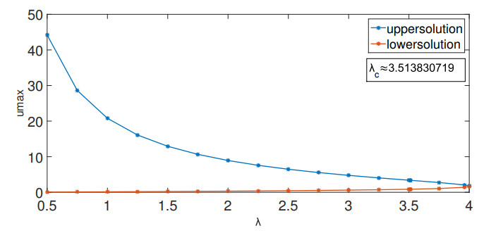
In this paper, we used the nonstandard compact finite difference method to numerically solve one-dimensional truncated Bratu-Picard equations and discussed the convergence analysis of the proposed method. Depending on the parameters in the mentioned equation, it may have no solution, one solution, or two solutions; also, it may have infinitely many solutions. The numerical results show that our method covers all mentioned aspects depending on the parameters in the equation.
- truncated Bratu–Picard model,
- boundary value problems,
- nonstandard compact finite difference methods
Citation: Maryam Arabameri, Raziyeh Gharechahi, Taher A. Nofal, Hijaz Ahmad. A nonstandard compact finite difference method for a truncated Bratu–Picard model[J]. AIMS Mathematics, 2024, 9(10): 27557-27576. doi: 10.3934/math.20241338

Related Papers:

Abstract

In this paper, we used the nonstandard compact finite difference method to numerically solve one-dimensional truncated Bratu-Picard equations and discussed the convergence analysis of the proposed method. Depending on the parameters in the mentioned equation, it may have no solution, one solution, or two solutions; also, it may have infinitely many solutions. The numerical results show that our method covers all mentioned aspects depending on the parameters in the equation.

References

[1]	R. Buckmire, Application of a Mickens finite-difference scheme to the cylindrical Bratu-Gelfand problem, Numer. Methods Partial Differ. Equ., 20 (2004), 327–337. https://doi.org/10.1002/num.10093 doi: 10.1002/num.10093
[2]	J. S. McGough, Numerical continuation and the Gelfand problem, Appl. Math. Comput., 89 (1998), 225–239. https://doi.org/10.1016/S0096-3003(97)81660-8 doi: 10.1016/S0096-3003(97)81660-8
[3]	H. Ahmad, R. Nawaz, F. Zia, M. Farooq, B. Almohsen, Application of novel method to withdrawal of thin film flow of a magnetohydrodynamic third grade fluid, Ain Shams Eng. J., 14 (2024), 102885. https://doi.org/10.1016/j.asej.2024.102885 doi: 10.1016/j.asej.2024.102885
[4]	M. I. Syam, A. Hamdan, An efficient method for solving Bratu equations, Appl. Math. Comput., 176 (2006), 704–713. https://doi.org/10.1016/j.amc.2005.10.021 doi: 10.1016/j.amc.2005.10.021
[5]	A. Akgul, H. Ahmad, Reproducing kernel method for Fangzhu's oscillator for water collection from air, Math. Methods Appl. Sci., 2020. https://doi.org/10.1002/mma.6853
[6]	A. M. Wazwaz, Adomian decomposition method for a reliable treatment of the Bratu-type equations, Appl. Math. Comput., 166 (2005), 652–663. https://doi.org/10.1016/j.amc.2004.06.059 doi: 10.1016/j.amc.2004.06.059
[7]	J. H. He, Some asymptotic methods for strongly nonlinear equations, Int. J. Mod. Phys. B, 20 (2006), 1141–1199. https://doi.org/10.1142/S0217979206033796 doi: 10.1142/S0217979206033796
[8]	J. H. He, Variational approach to the Bratu's problem, J. Phys. Conf. Ser., 96 (2008), 012087. https://doi.org/10.1088/1742-6596/96/1/012087 doi: 10.1088/1742-6596/96/1/012087
[9]	S. Liao, Y. Tan, A general approach to obtain series solutions of nonlinear differential equations, Stud. Appl. Math., 119 (2007), 297–354. https://doi.org/10.1111/j.1467-9590.2007.00387.x doi: 10.1111/j.1467-9590.2007.00387.x
[10]	M. Abdelhakem, H. Moussa, Pseudo-spectral matrices as a numerical tool for dealing BVPs, based on Legendre polynomials' derivatives, Alex. Eng. J., 66 (2023), 301–313. https://doi.org/10.1016/j.aej.2022.11.006 doi: 10.1016/j.aej.2022.11.006
[11]	M. Abdelhakem, D. Baleanu, P. Agarwal, H. Moussa, Approximating system of ordinary differential-algebraic equations via derivative of Legendre polynomials operational matrices, Int. J. Mod. Phys. C, 34 (2023), 2350036. https://doi.org/10.1142/S0129183123500365 doi: 10.1142/S0129183123500365
[12]	M. Abdelhakem, M. Fawzy, M. El-Kady, H. Moussa, An efficient technique for approximated BVPs via the second derivative Legendre polynomials pseudo-Galerkin method: certain types of applications, Results Phys., 43 (2022), 106067. https://doi.org/10.1016/j.rinp.2022.106067 doi: 10.1016/j.rinp.2022.106067
[13]	A. J. Ali, A. F. Abbas, M. A. Abdelhakem, Comparative analysis of Adams-Bashforth-Moulton and Runge-Kutta methods for solving ordinary differential equations using MATLAB, Math. Model. Eng. Probl., 11 (2024), 641–647. http://doi.org/10.18280/mmep.110307 doi: 10.18280/mmep.110307
[14]	M. Abdelhakem, Y. H. Youssri, Two spectral legendre's derivative algorithms for Lane-Emden, Bratu equations, and singular perturbed problems, Appl. Numer. Math., 169 (2021), 243–255. https://doi.org/10.1016/j.apnum.2021.07.006 doi: 10.1016/j.apnum.2021.07.006
[15]	S. A. Khuri, A new approach to Bratu's problem, Appl. Math. Comput., 147 (2004), 131–136. https://doi.org/10.1016/S0096-3003(02)00656-2 doi: 10.1016/S0096-3003(02)00656-2
[16]	S. Abbasbandy, M. S. Hashemi, C. S. Liu, The Lie-group shooting method for solving the Bratu equation, Commun. nonlinear Sci. Numer. Simul., 16 (2011), 4238–4249. https://doi.org/10.1016/j.cnsns.2011.03.033 doi: 10.1016/j.cnsns.2011.03.033
[17]	P. Korman, Y. Li, T. Ouyang, Exact multiplicity results for boundary value problems with nonlinearities generalizing cubic, Proc. Roy. Soc. Edinb.: Sec. A Math., 126 (1996), 599–616. https://doi.org/10.1017/S0308210500022927 doi: 10.1017/S0308210500022927
[18]	A. Mohsen, L. F. Sedeck, S. A. Mohamed, New smoother to enhanced multigrid-based methods for the Bratu problem, Appl. Math. Comput., 204 (2008), 325–339. https://doi.org/10.1016/j.amc.2008.06.058 doi: 10.1016/j.amc.2008.06.058
[19]	J. P. Boyd, One-point pseudo spectral collocation for the one dimensional Bratu equation, Appl. Math. Comput., 217 (2011), 5553–5565. https://doi.org/10.1016/j.amc.2010.12.029 doi: 10.1016/j.amc.2010.12.029
[20]	U. Erdogan, T. Ozis, A smart nonstandard finite difference scheme for second order nonlinear boundary value problems, J. Comput. Phys., 230 (2011), 6464–6574. https://doi.org/10.1016/j.jcp.2011.04.033 doi: 10.1016/j.jcp.2011.04.033
[21]	A. S. Mounim, B. M. de Dormale, From the fitting technique to accurate schemes for the Liouville-Bratu-Gelfand problem, Numer. Methods Partial Differ. Equ., 22 (2006), 761–775. https://doi.org/10.1002/num.20116 doi: 10.1002/num.20116
[22]	R. Gharechahi, M. Arab Ameri, M. Bisheh-Niasar, High order compact finite difference schemes for solving Bratu-type equations, J. Comput. Appl. Mech., 5 (2019), 91–102. https://doi.org/10.22055/JACM.2018.25696.1288 doi: 10.22055/JACM.2018.25696.1288
[23]	P. A. Zegeling, S. Iqbal, Nonstandard finite differences for a truncated Bratu–Picard model, Appl. Math. Comput., 324 (2018), 266–284. https://doi.org/10.1016/j.amc.2017.12.005 doi: 10.1016/j.amc.2017.12.005
[24]	P. G. Zhang, J. P. Wang, A predictor-corrector compact finite difference scheme for Burgers' equation, Appl. Math. Comput., 219 (2012), 892–898. https://doi.org/10.1016/j.amc.2012.06.064 doi: 10.1016/j.amc.2012.06.064
[25]	R. Mickens, Difference equation models of differential equations having zero local truncation errors, North-Holland Math. Stud., 92 (1984), 445–449. https://doi.org/10.1016/S0304-0208(08)73728-9 doi: 10.1016/S0304-0208(08)73728-9
[26]	R. Mickens, Nonstandard finite difference models of differential equations, World Scientific, 1993. https://doi.org/10.1142/2081
[27]	A. Mohsen, A simple solution of the Bratu problem, Comput. Math. Appl., 67 (2014), 26–33. https://doi.org/10.1016/j.camwa.2013.10.003 doi: 10.1016/j.camwa.2013.10.003

Reader Comments

Your name:*

Email:*
© 2024 the Author(s), licensee AIMS Press. This is an open access article distributed under the terms of the Creative Commons Attribution License (http://creativecommons.org/licenses/by/4.0)