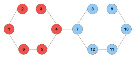
A satisfactory partition is a partition of undirected-graph vertices such that the partition has only two nonempty parts, and every vertex has at least as many adjacent vertices in its part as it has in the other part. Generally, the problem of determining whether a given undirected graph has a satisfactory partition is known to be NP-complete. In this paper, we show that for a given undirected graph with $ n $ vertices, a satisfactory partition (if any exists) can be computed recursively with a recursion tree of depth of $ \mathcal{O}(\ln n) $ in expectation. Subsequently, we show that a satisfactory partition for those undirected graphs with recursion tree depth meeting the expectation can be computed in time $ \mathcal{O}(n^{3} 2^{\mathcal{O}(\ln n)}) $.
Citation: Samer Nofal. On finding a satisfactory partition in an undirected graph: algorithm design and results[J]. AIMS Mathematics, 2024, 9(10): 27308-27329. doi: 10.3934/math.20241327
A satisfactory partition is a partition of undirected-graph vertices such that the partition has only two nonempty parts, and every vertex has at least as many adjacent vertices in its part as it has in the other part. Generally, the problem of determining whether a given undirected graph has a satisfactory partition is known to be NP-complete. In this paper, we show that for a given undirected graph with $ n $ vertices, a satisfactory partition (if any exists) can be computed recursively with a recursion tree of depth of $ \mathcal{O}(\ln n) $ in expectation. Subsequently, we show that a satisfactory partition for those undirected graphs with recursion tree depth meeting the expectation can be computed in time $ \mathcal{O}(n^{3} 2^{\mathcal{O}(\ln n)}) $.

| [1] |
M. U. Gerber, D. Kobler, Algorithmic approach to the satisfactory graph partitioning problem, Eur. J. Oper. Res., 125 (2000), 283–291. https://doi.org/10.1016/S0377-2217(99)00459-2 doi: 10.1016/S0377-2217(99)00459-2

|
| [2] |
M. U. Gerber, D. Kobler, Algorithms for vertex-partitioning problems on graphs with fixed clique-width, Theor. Comput. Sci., 299 (2003), 719–734. https://doi.org/10.1016/S0304-3975(02)00725-9 doi: 10.1016/S0304-3975(02)00725-9
|
| [3] | C. Bazgan, Z. Tuza, D. Vanderpooten, On the existence and determination of satisfactory partitions in a graph, In: T. Ibaraki, N. Katoh, H. Ono, Algorithms and computation, Springer-Verlag, 2003. https://doi.org/10.1007/978-3-540-24587-2_46 |
| [4] |
C. Bazgan, Z. Tuza, D. Vanderpooten, The satisfactory partition problem, Discrete Appl. Math., 154 (2006), 1236–1245. https://doi.org/10.1016/j.dam.2005.10.014 doi: 10.1016/j.dam.2005.10.014
|
| [5] | C. Bazgan, Z. Tuza, D. Vanderpooten, Complexity and approximation of satisfactory partition problems, In: L. Wang, Computing and combinatorics, Springer-Verlag, 2005. https://doi.org/10.1007/11533719_84 |
| [6] |
A. Gaikwad, S. Maity, S. K. Tripathi, Parameterized complexity of satisfactory partition problem, Theor. Comput. Sci., 907 (2022), 113–127. https://doi.org/10.1016/j.tcs.2022.01.022 doi: 10.1016/j.tcs.2022.01.022
|
| [7] |
N. Kim, Z. Zheng, S. Elmetwaly, T. Schlick, Rna graph partitioning for the discovery of rna modularity: a novel application of graph partition algorithm to biology, Plos One, 9 (2014), e106074. https://doi.org/10.1371/journal.pone.0106074 doi: 10.1371/journal.pone.0106074
|
| [8] | L. Jäntschi, M. V. Diudea, Subgraphs of pair vertices, J. Math. Chem., 45 (2009), 364–371. https://doi.org/10.1007/s10910-008-9411-6 |
| [9] |
C. Guada, E. Zarrazola, J. Yáñez, J. T. Rodríguez, D. Gómez, J. Montero, A novel edge detection algorithm based on a hierarchical graph-partition approach, J. Intell. Fuzzy Syst., 34 (2018), 1875–1892. https://doi.org/10.3233/JIFS-171218 doi: 10.3233/JIFS-171218
|
| [10] |
M. Li, H. Cui, C. Zhou, S. Xu, Gap: genetic algorithm based large-scale graph partition in heterogeneous cluster, IEEE Access, 8 (2020), 144197–144204. https://doi.org/10.1109/ACCESS.2020.3014351 doi: 10.1109/ACCESS.2020.3014351
|
| [11] |
H. Cui, D. Yang, C. Zhou, A large-scale graph partition algorithm with redundant multi-order neighbor vertex storage, Inf. Sci., 667 (2024), 120473. https://doi.org/10.1016/j.ins.2024.120473 doi: 10.1016/j.ins.2024.120473
|
| [12] |
H. Li, R. Fu, X. Ma, Forbidden subgraphs in reduced power graphs of finite groups, AIMS Math., 6 (2021), 5410–5420. https://doi.org/10.3934/math.2021319 doi: 10.3934/math.2021319
|
| [13] |
S. Fidanova, P. C. Pop, An improved hybrid ant-local search algorithm for the partition graph coloring problem, J. Comput. Appl. Math., 293 (2016), 55–61. https://doi.org/10.1016/j.cam.2015.04.030 doi: 10.1016/j.cam.2015.04.030
|
| [14] | S. Fidanova, P. C. Pop, An ant algorithm for the partition graph coloring problem, In: I. Dimov, S. Fidanova, I. Lirkov, Numerical methods and applications, Springer-Verlag, 2014. https://doi.org/10.1007/978-3-319-15585-2_9 |
| [15] | S. Zhang, Z. Jiang, X. Hou, Z. Guan, M. Yuan, H. You, An efficient and balanced graph partition algorithm for the subgraph-centric programming model on large-scale power-law graphs, 2021 IEEE 41st International Conference on Distributed Computing Systems (ICDCS), 2021. https://doi.org/10.1109/ICDCS51616.2021.00016 |
| [16] | L. Chen, Y. Chen, Y. Wang, An improved spectral graph partition intelligent clustering algorithm for low-power wireless networks, J. Ambient Intell. Humanized Comput., 2019. https://doi.org/10.1007/s12652-019-01508-7 |
| [17] |
Y. Leng, H. Wang, F. Lu, Artificial intelligence knowledge graph for dynamic networks: an incremental partition algorithm, IEEE Access, 8 (2020), 63434–63442. https://doi.org/10.1109/ACCESS.2020.2982652 doi: 10.1109/ACCESS.2020.2982652
|
| [18] |
X. Heng, Y. Chen, L. Liu, Medical intelligent system and orthopedic clinical nursing based on graph partition sampling algorithm, Comput. Intell. Neurosci., 2022 (2022), 2764157. https://doi.org/10.1155/2022/2764157 doi: 10.1155/2022/2764157
|
| [19] |
L. Wang, S. Ding, Y. Wang, L. Ding, A robust spectral clustering algorithm based on grid-partition and decision-graph, Int. J. Mach. Learn. Cybern., 12 (2021), 1243–1254. https://doi.org/10.1007/s13042-020-01231-2 doi: 10.1007/s13042-020-01231-2
|
| [20] |
J. Wang, Y. Guo, X. Wen, Z. Wang, Z. Li, M. Tang, Improving graph-based label propagation algorithm with group partition for fraud detection, Appl. Intell., 50 (2020), 3291–3300. https://doi.org/10.1007/s10489-020-01724-1 doi: 10.1007/s10489-020-01724-1
|
| [21] |
M. Fu, Y. Zhang, Results on monochromatic vertex disconnection of graphs, AIMS Math., 8 (2023), 13219–13240. https://doi.org/10.3934/math.2023668 doi: 10.3934/math.2023668
|
| [22] | W. Zhou, H. Tang, Z. Ji, A task partition algorithm based on grid and graph partition for distributed crowd simulation, 2014 Fourth International Conference on Instrumentation and Measurement, Computer, Communication and Control, 2014. https://doi.org/10.1109/IMCCC.2014.113 |
| [23] | J. W. Zhan, A novel sports video background segmentation algorithm based on graph partition, 2015 8th International Conference on Intelligent Computation Technology and Automation (ICICTA), 2015. https://doi.org/10.1109/ICICTA.2015.25 |
| [24] |
H. Cui, Y. Wu, S. Lv, Property graph partition algorithm based on improved barnacle mating optimization, J. Phys., 2832 (2024), 012005. https://doi.org/10.1088/1742-6596/2832/1/012005 doi: 10.1088/1742-6596/2832/1/012005
|
| [25] | Y. Chen, Q. Wang, X. Cai, N. Wang, A new text mining method of dispatching operation ticket system based on graph partition spectral clustering algorithm, 2023 6th International Conference on Energy, Electrical and Power Engineering (CEEPE), 2023, 1517–1521. https://doi.org/10.1109/CEEPE58418.2023.10166981 |
| [26] |
B. Ma, C. Yang, Distinguishing colorings of graphs and their subgraphs, AIMS Math., 8 (2023), 26561–26573. https://doi.org/10.3934/math.20231357 doi: 10.3934/math.20231357
|
| [27] | S. Luo, L. Liu, H. Wang, B. Wu, Y. Liu, Implementation of a parallel graph partition algorithm to speed up bsp computing, 2014 11th International Conference on Fuzzy Systems and Knowledge Discovery (FSKD), 2014. https://doi.org/10.1109/FSKD.2014.6980928 |
| [28] | P. C. Pop, B. Hu, G. R. Raidl, A memetic algorithm with two distinct solution representations for the partition graph coloring problem, In: R. M. Díaz, F. Pichler, A. Q. Arencibia, Computer aided systems theory-EUROCAST, Springer-Verlag, 2013. https://doi.org/10.1007/978-3-642-53856-8_28 |
| [29] |
L. Jäntschi, S. D. Bolboacă, Informational entropy of b-ary trees after a vertex cut, Entropy, 10 (2008), 576–588. https://doi.org/10.3390/e10040576 doi: 10.3390/e10040576
|
| [30] |
W. Zhao, Y. Li, R. Lin, The existence of a graph whose vertex set can be partitioned into a fixed number of strong domination-critical vertex-sets, AIMS Math., 9 (2024), 1926–1938. https://doi.org/10.3934/math.2024095 doi: 10.3934/math.2024095
|
| [31] |
J. Gómez-Gardeñes, E. Estrada, Network bipartitioning in the anti-communicability euclidean space, AIMS Math., 6 (2021), 1153–1174. https://doi.org/10.3934/math.2021070 doi: 10.3934/math.2021070
|
| [32] |
S. D. Bolboacă, L. Jäntschi, Nanoquantitative structure-property relationship modeling on $c_42$ fullerene isomers, J. Chem., 2016 (2016), 1791756. https://doi.org/10.1155/2016/1791756 doi: 10.1155/2016/1791756
|
| [33] |
D. M. Joiţa, L. Jäntschi, Extending the characteristic polynomial for characterization of $c_20$ fullerene congeners, Mathematics, 5 (2017), 84. https://doi.org/10.3390/math5040084 doi: 10.3390/math5040084
|
Figures(2)

Samer Nofal. On finding a satisfactory partition in an undirected graph: algorithm design and results[J]. AIMS Mathematics, 2024, 9(10): 27308-27329. doi: 10.3934/math.20241327


 DownLoad: