A chemostat is a laboratory device (of the bioreactor type) in which organisms (bacteria, phytoplankton) develop in a controlled manner. This paper studies the asymptotic properties of a chemostat model with generalized interference function and Poisson noise. Due to the complexity of abrupt and erratic fluctuations, we consider the effect of the second order Itô-Lévy processes. The dynamics of our perturbed system are determined by the value of the threshold parameter $ \mathfrak{C}^{\star}_0 $. If $ \mathfrak {C}^{\star}_0 $ is strictly positive, the stationarity and ergodicity properties of our model are verified (practical scenario). If $ \mathfrak {C}^{\star}_0 $ is strictly negative, the considered and modeled microorganism will disappear in an exponential manner. This research provides a comprehensive overview of the chemostat interaction under general assumptions that can be applied to various models in biology and ecology. In order to verify the reliability of our results, we probe the case of industrial waste-water treatment. It is concluded that higher order jumps possess a negative influence on the long-term behavior of microorganisms in the sense that they lead to complete extinction.
Citation: Yassine Sabbar, José Luis Diaz Palencia, Mouhcine Tilioua, Abraham Otero, Anwar Zeb, Salih Djilali. A general chemostat model with second-order Poisson jumps: asymptotic properties and application to industrial waste-water treatment[J]. AIMS Mathematics, 2023, 8(6): 13024-13049. doi: 10.3934/math.2023656
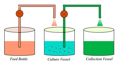
A chemostat is a laboratory device (of the bioreactor type) in which organisms (bacteria, phytoplankton) develop in a controlled manner. This paper studies the asymptotic properties of a chemostat model with generalized interference function and Poisson noise. Due to the complexity of abrupt and erratic fluctuations, we consider the effect of the second order Itô-Lévy processes. The dynamics of our perturbed system are determined by the value of the threshold parameter $ \mathfrak{C}^{\star}_0 $. If $ \mathfrak {C}^{\star}_0 $ is strictly positive, the stationarity and ergodicity properties of our model are verified (practical scenario). If $ \mathfrak {C}^{\star}_0 $ is strictly negative, the considered and modeled microorganism will disappear in an exponential manner. This research provides a comprehensive overview of the chemostat interaction under general assumptions that can be applied to various models in biology and ecology. In order to verify the reliability of our results, we probe the case of industrial waste-water treatment. It is concluded that higher order jumps possess a negative influence on the long-term behavior of microorganisms in the sense that they lead to complete extinction.

| [1] | H. L. Smith, P. Waltman, The theory of the chemostat: dynamics of microbial competition, Cambridge: Cambridge university press, 1995. |
| [2] | W. Nazaroff, L. Alvarez-Cohen, Environmental engineering science, New York: John Wiley and Sons, 2001. |
| [3] |
A. Novick, L. Szilard, Experiments with the chemostat on spontaneous mutations of bacteria, Proc. Natl. Acad. Sci., 36 (1950), 708–719. https://doi.org/10.1073/pnas.36.12.708 doi: 10.1073/pnas.36.12.708

|
| [4] |
A. Novick, L. Szilard, Description of the chemostat, Science, 112 (1950), 715–716. https://doi.org/10.1126/science.112.2920.715 doi: 10.1126/science.112.2920.715
|
| [5] |
S. Pavlou, I. G. Kevrekidis, Microbial predation in a periodically operated chemostat: a global study of the interaction between natural and externally imposed frequencies, Math. Biosci., 108 (1992), 1–55. https://doi.org/10.1016/0025-5564(92)90002-E doi: 10.1016/0025-5564(92)90002-E
|
| [6] |
F. Y. Wang, G. P. Pang, S. W. Zhang, Analysis of a Lotka-Volterra food chain chemostat with converting time delays, Chaos Soliton. Fract., 42 (2009), 2786–2795. https://doi.org/10.1016/j.chaos.2009.03.189 doi: 10.1016/j.chaos.2009.03.189
|
| [7] |
G. P. Pang, F. Y. Wang, L. S. Chen, Study of Lotka-Volterra food chain chemostat with periodically varying dilution rate, J. Math. Chem., 43 (2008), 901–913. https://doi.org/10.1007/s10910-007-9263-5 doi: 10.1007/s10910-007-9263-5
|
| [8] | J. Monod, La technique de culture continue: theorie et applications, Ann. Inst. Pasteur., 79 (1950), 390–410. |
| [9] | J. Monod, Recherches sur la croissance des cultures bacteriennes, Hermann, 1942. |
| [10] |
G. S. K. Wolkowicz, Z. Q. Lu, Global dynamics of a mathematical model of competition in the chemostat: general response functions and differential death rates, SIAM J. Appl. Math., 52 (1992), 222–233. https://doi.org/10.1137/0152012 doi: 10.1137/0152012
|
| [11] |
B. T. Li, Global asymptotic behavior of the chemostat: general response functions and different removal rates, SIAM J. Appl. Math., 59 (1998), 411–422. https://doi.org/10.1137/S003613999631100X doi: 10.1137/S003613999631100X
|
| [12] |
B. Tang, G. Wolkowicz, Mathematical models of microbial growth and competition in the chemostat regulated by cell-bound extracellular enzymes, J. Math. Biol., 31 (1992), 1–23. https://doi.org/10.1007/BF00163841 doi: 10.1007/BF00163841
|
| [13] |
A. Rapaport, J. Harmand, Biological control of the chemostat with nonmonotonic response and different removal rates, Math. Biosci. Eng., 5 (2008), 539–547. https://doi.org/10.3934/mbe.2008.5.539 doi: 10.3934/mbe.2008.5.539
|
| [14] |
F. Mazenc, M. Malisoff, Stabilization of a chemostat model with haldane growth functions and a delay in the measurements, Automatica, 46 (2010), 1428–1436. https://doi.org/10.1016/j.automatica.2010.06.012 doi: 10.1016/j.automatica.2010.06.012
|
| [15] |
J. F. Andrews, A mathematical model for the continuous culture of microorganisms utilizing inhibitory substrates, Biotechnol. Bioeng., 10 (1968), 707–723. https://doi.org/10.1002/bit.260100602 doi: 10.1002/bit.260100602
|
| [16] |
Y. Sabbar, A. Zeb, N. Gul, D. Kiouach, S. Rajasekar, N. Ullah, et al., Stationary distribution of an sir epidemic model with three correlated brownian motions and general lévy measure, AIMS Mathematics, 8 (2023), 1329–1344. https://doi.org/10.3934/math.2023066 doi: 10.3934/math.2023066
|
| [17] |
Y. Sabbar, D. Kiouach, S. P. Rajasekar, Acute threshold dynamics of an epidemic system with quarantine strategy driven by correlated white noises and Lévy jumps associated with infinite measure, International Journal of Dynamics and Control, 11 (2023), 122–135. https://doi.org/10.1007/s40435-022-00981-x doi: 10.1007/s40435-022-00981-x
|
| [18] |
Y. Sabbar, M. Yavuz, F. Ozkose, Infection eradication criterion in a general epidemic model with logistic growth, quarantine strategy, media intrusion, and quadratic perturbation, Mathematics, 10 (2022), 4213. https://doi.org/10.3390/math10224213 doi: 10.3390/math10224213
|
| [19] |
A. Din, A. Khan, Y. Sabbar, Long-term bifurcation and stochastic optimal control of a triple-delayed ebola virus model with vaccination and quarantine strategies, Fractal Fract., 6 (2022), 578. https://doi.org/10.3390/fractalfract6100578 doi: 10.3390/fractalfract6100578
|
| [20] |
D. L. Zhao, S. L. Yuan, Sharp conditions for the existence of a stationary distribution in one classical stochastic chemostat, Appl. Math. Comput., 339 (2018), 199–205. https://doi.org/10.1016/j.amc.2018.07.020 doi: 10.1016/j.amc.2018.07.020
|
| [21] |
M. M. Gao, D. Q. Jiang, T. Hayat, A. Alsaedi, Threshold behavior of a stochastic Lotka-Volterra food chain chemostat model with jumps, Physica A, 523 (2019), 191–203. https://doi.org/10.1016/j.physa.2019.02.029 doi: 10.1016/j.physa.2019.02.029
|
| [22] |
X. J. Lv, X. Z. Meng, X. Z. Wang, Extinction and stationary distribution of an impulsive stochastic chemostat model with nonlinear perturbation, Chaos Soliton. Fract., 110 (2018), 273–279. https://doi.org/10.1016/j.chaos.2018.03.038 doi: 10.1016/j.chaos.2018.03.038
|
| [23] |
A. Khan, Y. Sabbar, A. Din, Stochastic modeling of the Monkeypox 2022 epidemic with cross-infection hypothesis in a highly disturbed environment, Math. Biosci. Eng., 19 (2022), 13560–13581. https://doi.org/10.3934/mbe.2022633 doi: 10.3934/mbe.2022633
|
| [24] |
Y. Sabbar, A. Khan, A. Din, Probabilistic analysis of a marine ecological system with intense variability, Mathematics, 10 (2022), 2262. https://doi.org/10.3390/math10132262 doi: 10.3390/math10132262
|
| [25] |
Y. Sabbar, A. Khan, A. Din, D. Kiouach, S. P. Rajasekar, Determining the global threshold of an epidemic model with general interference function and high-order perturbation, AIMS Mathematics, 7 (2022), 19865–19890. https://doi.org/10.3934/math.20221088 doi: 10.3934/math.20221088
|
| [26] |
D. L. Zhao, S. L. Yuan, H. D. Liu, Stochastic dynamics of the delayed chemostat with Levy noises, Int. J. Biomath., 12 (2019), 1950056. https://doi.org/10.1142/S1793524519500566 doi: 10.1142/S1793524519500566
|
| [27] |
X. F. Zhang, R. Yuan, A stochastic chemostat model with mean-reverting Ornstein-Uhlenbeck process and Monod-Haldane response function, Appl. Math. Comput., 394 (2021), 125833. https://doi.org/10.1016/j.amc.2020.125833 doi: 10.1016/j.amc.2020.125833
|
| [28] |
Z. W. Cao, X. D. Wen, H. S. Su, L. Y. Liu, Q. Ma, Stationary distribution of a stochastic chemostat model with Beddington-Deangelis functional response, Physica A, 554 (2020), 124634. https://doi.org/10.1016/j.physa.2020.124634 doi: 10.1016/j.physa.2020.124634
|
| [29] |
Y. Sabbar, D. Kiouach, S. P. Rajasekar, S. E. A. El-Idrissi, The influence of quadratic Lévy noise on the dynamic of an SIC contagious illness model: new framework, critical comparison and an application to COVID-19 (SARA-CoV-2) case, Chaos Soliton. Fract., 159 (2022), 112110. https://doi.org/10.1016/j.chaos.2022.112110 doi: 10.1016/j.chaos.2022.112110
|
| [30] |
D. Kiouach, Y. Sabbar, The long-time behaviour of a stochastic SIR epidemic model with distributed delay and multidimensional Levy jumps, Int. J. Biomath., 15 (2022), 2250004. https://doi.org/10.1142/S1793524522500048 doi: 10.1142/S1793524522500048
|
| [31] |
D. Kiouach, Y. Sabbar, Developing new techniques for obtaining the threshold of a stochastic SIR epidemic model with 3-dimensional Levy process, Journal of Applied Nonlinear Dynamics, 11 (2022), 401–414. https://doi.org/10.5890/JAND.2022.06.010 doi: 10.5890/JAND.2022.06.010
|
| [32] |
D. Kiouach, Y. Sabbar, S. E. A. El-idrissi, New results on the asymptotic behavior of an SIS epidemiological model with quarantine strategy, stochastic transmission, and Levy disturbance, Math. Method. Appl. Sci., 44 (2021), 13468–13492. https://doi.org/10.1002/mma.7638 doi: 10.1002/mma.7638
|
| [33] |
X. H. Zhang, K. Wang, Stochastic SIR model with jumps, Appl. Math. Lett., 26 (2013), 867–874. https://doi.org/10.1016/j.aml.2013.03.013 doi: 10.1016/j.aml.2013.03.013
|
| [34] |
Y. L. Zhou, W. G. Zhang, Threshold of a stochastic SIR epidemic model with Levy jumps, Physica A, 446 (2016), 204–216. https://doi.org/10.1016/j.physa.2015.11.023 doi: 10.1016/j.physa.2015.11.023
|
| [35] |
D. Kiouach, Y. Sabbar, Developing new techniques for obtaining the threshold of a stochastic SIR epidemic model with 3-dimensional Levy process, Journal of Applied Nonlinear Dynamics, 11 (2022), 401–414. https://doi.org/10.5890/JAND.2022.06.010 doi: 10.5890/JAND.2022.06.010
|
| [36] |
D. Kiouach, Y. Sabbar, The long-time behaviour of a stochastic SIR epidemic model with distributed delay and multidimensional Levy jumps, Int. J. Biomath., 15 (2022), 2250004. https://doi.org/10.1142/S1793524522500048 doi: 10.1142/S1793524522500048
|
| [37] |
D. Kiouach, Y. Sabbar, Dynamic characterization of a stochastic SIR infectious disease model with dual perturbation, Int. J. Biomath., 14 (2021), 2150016. https://doi.org/10.1142/S1793524521500169 doi: 10.1142/S1793524521500169
|
| [38] | I. I. Gihman, A. V. Skorohod, Stochastic differential equations, Berlin Heidelberg: Springer, 1972. |
| [39] |
Y. Cheng, F. M. Zhang, M. Zhao, A stochastic model of HIV infection incorporating combined therapy of HARRT driven by Levy jumps, Adv. Differ. Equ., 2019 (2019), 321. https://doi.org/10.1186/s13662-019-2108-2 doi: 10.1186/s13662-019-2108-2
|
| [40] |
Y. Cheng, M. T. Li, F. M. Zhang, A dynamics stochastic model with HIV infection of CD4+ T-cells driven by Levy noise, Chaos Soliton. Fract., 129 (2019), 62–70. https://doi.org/10.1016/j.chaos.2019.07.054 doi: 10.1016/j.chaos.2019.07.054
|
| [41] |
N. T. Dieu, T. Fugo, N. H. Du, Asymptotic behaviors of stochastic epidemic models with jump-diffusion, Appl. Math. Model., 86 (2020), 259–270. https://doi.org/10.1016/j.apm.2020.05.003 doi: 10.1016/j.apm.2020.05.003
|
| [42] |
N. Privault, L. Wang, Stochastic SIR Levy jump model with heavy tailed increments, J. Nonlinear Sci., 31 (2021), 15. https://doi.org/10.1007/s00332-020-09670-5 doi: 10.1007/s00332-020-09670-5
|
| [43] |
G. J. Butler, G. S. K. Wolkowicz, A mathematical model of the chemostat with a general class of functions describing nutrient uptake, SIAM J. Appl. Math., 45 (1985), 138–151. https://doi.org/10.1137/0145006 doi: 10.1137/0145006
|
| [44] |
Q. L. Dong, W. B. Ma, M. J. Sun, The asymptotic behavior of a chemostat model with crowley-martin type functional response and time delays, J. Math. Chem., 51 (2013), 1231–1248. https://doi.org/10.1007/s10910-012-0138-z doi: 10.1007/s10910-012-0138-z
|
| [45] |
H. X. Li, J. H. Wu, Y. L. Li, C. A. Liu, Positive solutions to the unstirred chemostat model with crowley-martin functional response, AIMS Mathematics, 23 (2018), 2951–2966. https://doi.org/10.3934/dcdsb.2017128 doi: 10.3934/dcdsb.2017128
|
| [46] |
L. Wang, D. Q. Jiang, Ergodic property of the chemostat: a stochastic model under regime switching and with general response function, Nonlinear Analysis: Hybrid Systems, 27 (2018), 341–352. https://doi.org/10.1016/j.nahs.2017.10.001 doi: 10.1016/j.nahs.2017.10.001
|
| [47] |
L. Wang, D. Q. Jiang, A note on the stationary distribution of the stochastic chemostat model with general response functions, Appl. Math. Lett., 73 (2017), 22–28. https://doi.org/10.1016/j.aml.2017.04.029 doi: 10.1016/j.aml.2017.04.029
|
| [48] |
Y. Sabbar, A. Khan, A. Din, M. Tilioua, New method to investigate the impact of independent quadratic alpha-stable Poisson jumps on the dynamics of a disease under vaccination strategy, Fractal Fract., 7 (2023), 226. https://doi.org/10.3390/fractalfract7030226 doi: 10.3390/fractalfract7030226
|
| [49] |
Y. Sabbar, A. Zeb, D. Kiouach, N. Gul, T. Sitthiwirattham, D. Baleanu, et al., Dynamical bifurcation of a sewage treatment model with general higher-order perturbation, Results Phys., 39 (2022), 105799. https://doi.org/10.1016/j.rinp.2022.105799 doi: 10.1016/j.rinp.2022.105799
|
| [50] |
Q. Liu, D. Q. Jiang, T. Hayat, B. Ahmed, Periodic solution and stationary distribution of stochastic SIR epidemic models with higher order perturbation, Physica A, 482 (2017), 209–217. https://doi.org/10.1016/j.physa.2017.04.056 doi: 10.1016/j.physa.2017.04.056
|
| [51] |
Q. Liu, D. Q. Jiang, Stationary distribution and extinction of a stochastic SIR model with nonlinear perturbation, Appl. Math. Lett., 73 (2017), 8–15. https://doi.org/10.1016/j.aml.2017.04.021 doi: 10.1016/j.aml.2017.04.021
|
| [52] |
Q. Liu, D. Q Jiang, T. Hayat, B. Ahmed, Stationary distribution and extinction of a stochastic predator-prey model with additional food and nonlinear perturbation, Appl. Math. Comput., 320 (2018), 226–239. https://doi.org/10.1016/j.amc.2017.09.030 doi: 10.1016/j.amc.2017.09.030
|
| [53] |
S. G. Peng, X. H. Zhu, Necessary and sufficient condition for comparison theorem of 1-dimensional stochastic differential equations, Stoch. Proc. Appl., 116 (2006), 370–380. https://doi.org/10.1016/j.spa.2005.08.004 doi: 10.1016/j.spa.2005.08.004
|
| [54] |
N. T. Dieu, D. H. Nguyen, N. H. Du, G. Yin, Classification of asymptotic behavior in a stochastic SIR model, SIAM J. Appl. Dyn. Syst., 15 (2016), 1062–1084. https://doi.org/10.1137/15M1043315 doi: 10.1137/15M1043315
|
| [55] |
F. B. Xi, Asymptotic properties of jump-diffusion processes with state-dependent switching, Stoch. Proc. Appl., 119 (2009), 2198–2221. https://doi.org/10.1016/j.spa.2008.11.001 doi: 10.1016/j.spa.2008.11.001
|
| [56] | Y. A. Kutoyants, Statistical inference for ergodic diffusion processes, London: Springer, 2004. https://doi.org/10.1007/978-1-4471-3866-2 |
| [57] | L. Stettner, On the existence and uniqueness of invariant measure for continuous time Markov processes, Brown University, 1986. |
| [58] |
J. Y. Tong, Z. Z. Zhang, J. H. Bao, The stationary distribution of the facultative population model with a degenerate noise, Stat. Probabil. Lett., 83 (2013), 655–664. https://doi.org/10.1016/j.spl.2012.11.003 doi: 10.1016/j.spl.2012.11.003
|
| [59] | X. R. Mao, Stochastic differential equations and applications. Chichester: Elsevier, 2007. |
| [60] |
D. H. Nguyen, N. N. Nguyen, G. Yin, General nonlinear stochastic systems motivated by chemostat models: complete characterization of long time behavior, optimal controls, and applications to wastewater treatment, Stoch. Proc. Appl., 130 (2020), 4608–4642. https://doi.org/10.1016/j.spa.2020.01.010 doi: 10.1016/j.spa.2020.01.010
|
| [61] |
N. B. Liberati, E. Platen, Strong approximations of stochastic differential equations with jumps, J. Comput. Appl. Math., 205 (2007), 982–1001. https://doi.org/10.1016/j.cam.2006.03.040 doi: 10.1016/j.cam.2006.03.040
|


Figures(7) / Tables(5)

Yassine Sabbar, José Luis Diaz Palencia, Mouhcine Tilioua, Abraham Otero, Anwar Zeb, Salih Djilali. A general chemostat model with second-order Poisson jumps: asymptotic properties and application to industrial waste-water treatment[J]. AIMS Mathematics, 2023, 8(6): 13024-13049. doi: 10.3934/math.2023656


 DownLoad: