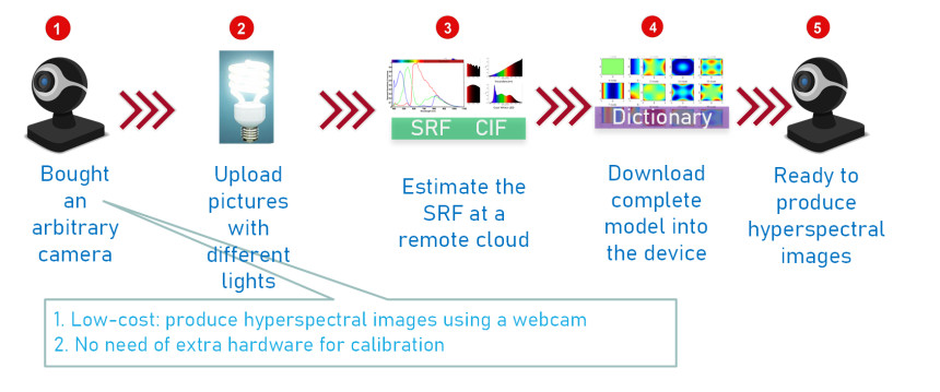
Synthesizing hyperspectral images (HSI) from an ordinary camera has been accomplished recently. However, such computation models require detailed properties of the target camera, which can only be measured in a professional lab. This prerequisite prevents the synthesizing model from being installed on arbitrary cameras for end-users. This study offers a calibration-free method for transforming any camera into an HSI camera. Our solution requires no controllable light sources and spectrometers. Any consumer installing the program should produce high-quality HSI without the assistance of optical laboratories. Our approach facilitates a cycle-generative adversarial network (cycle-GAN) and sparse assimilation method to render the illumination-dependent spectral response function (SRF) of the underlying camera at the first part of the setup stage. The current illuminating function (CIF) must be identified for each image and decoupled from the underlying model. The HSI model is then integrated with the static SRF and dynamic CIF in the second part of the stage. The estimated SRFs and CIFs have been double-checked with the results by the standard laboratory method. The reconstructed HSIs have errors under 3% in the root mean square.
Citation: Yenming J. Chen, Jinn-Tsong Tsai, Kao-Shing Hwang, Chin-Lan Chen, Wen-Hsien Ho. Intelligent synthesis of hyperspectral images from arbitrary web cameras in latent sparse space reconstruction[J]. AIMS Mathematics, 2023, 8(11): 27989-28009. doi: 10.3934/math.20231432
Synthesizing hyperspectral images (HSI) from an ordinary camera has been accomplished recently. However, such computation models require detailed properties of the target camera, which can only be measured in a professional lab. This prerequisite prevents the synthesizing model from being installed on arbitrary cameras for end-users. This study offers a calibration-free method for transforming any camera into an HSI camera. Our solution requires no controllable light sources and spectrometers. Any consumer installing the program should produce high-quality HSI without the assistance of optical laboratories. Our approach facilitates a cycle-generative adversarial network (cycle-GAN) and sparse assimilation method to render the illumination-dependent spectral response function (SRF) of the underlying camera at the first part of the setup stage. The current illuminating function (CIF) must be identified for each image and decoupled from the underlying model. The HSI model is then integrated with the static SRF and dynamic CIF in the second part of the stage. The estimated SRFs and CIFs have been double-checked with the results by the standard laboratory method. The reconstructed HSIs have errors under 3% in the root mean square.

| [1] | B. Arad, O. Ben-Shahar, Sparse recovery of hyperspectral signal from natural RGB images, in European Conference on Computer Vision, Springer, 19–34. (2016), https://doi.org/10.1007/978-3-319-46478-7_2 |
| [2] |
I. Choi, D. S. Jeon, G. Nam, D. Gutierrez, M. H. Kim, High-quality hyperspectral reconstruction using a spectral prior, ACM T. Graphic., 36 (2017), 1–13. http://dx.doi.org/10.1145/3130800.3130810 doi: 10.1145/3130800.3130810

|
| [3] |
W. Jakob, J. Hanika, A low-dimensional function space for efficient spectral upsampling, Comput. Graph. Forum, 38 (2019), 147–155. https://doi.org/10.1111/cgf.13626 doi: 10.1111/cgf.13626
|
| [4] | Y. Jia, Y. Zheng, L. Gu, A. Subpa-Asa, A. Lam, Y. Sato, et al., From RGB to spectrum for natural scenes via manifold-based mapping, in Proceedings of the IEEE international conference on computer vision, 4705–4713, (2017). https://doi.org/10.1109/ICCV.2017.504 |
| [5] | H. Kwon, Y. W. Tai, RGB-guided hyperspectral image upsampling, in Proceedings of the IEEE International Conference on Computer Vision, 307–315, (2015). https://doi.org/10.1109/ICCV.2015.43 |
| [6] | S. W. Oh, M. S. Brown, M. Pollefeys, S. J. Kim, Do it yourself hyperspectral imaging with everyday digital cameras, in Proceedings of the IEEE Conference on Computer Vision and Pattern Recognition, 2461–2469, (2016). https://doi.org/10.1109/CVPR.2016.270 |
| [7] |
Q. Li, X. He, Y. Wang, H. Liu, D. Xu, F. Guo, Review of spectral imaging technology in biomedical engineering: achievements and challenges, J. Biomed. Opt., 18 (2013), 100901–100901. https://doi.org/10.1117/1.JBO.18.10.100901 doi: 10.1117/1.JBO.18.10.100901
|
| [8] |
M. Aharon, M. Elad, A. Bruckstein, K-SVD: An algorithm for designing overcomplete dictionaries for sparse representation, IEEE T. Signal Proces., 54 (2006), 4311–4322. https://doi.org/10.1109/TSP.2006.881199 doi: 10.1109/TSP.2006.881199
|
| [9] |
Z. Xing, M. Zhou, A. Castrodad, G. Sapiro, L. Carin, Dictionary learning for noisy and incomplete hyperspectral images, SIAM J. Imag. Sci., 5 (2012), 33–56. https://doi.org/10.1137/110837486 doi: 10.1137/110837486
|
| [10] |
O. Burggraaff, N. Schmidt, J. Zamorano, K. Pauly, S. Pascual, C. Tapia, et al., Standardized spectral and radiometric calibration of consumer cameras, Optics Express, 27 (2019), 19075–19101. https://doi.org/10.1364/OE.27.019075 doi: 10.1364/OE.27.019075
|
| [11] | J. Jiang, D. Liu, J. Gu, S. Süsstrunk, What is the space of spectral sensitivity functions for digital color cameras?, in 2013 IEEE Workshop on Applications of Computer Vision (WACV), IEEE, 168–179, (2013). https://doi.org/10.1109/WACV.2013.6475015 |
| [12] | S. Han, Y. Matsushita, I. Sato, T. Okabe, Y. Sato, Camera spectral sensitivity estimation from a single image under unknown illumination by using fluorescence, in 2012 IEEE Conference on Computer Vision and Pattern Recognition, IEEE, 805–812, (2012). https://doi.org/10.1109/CVPR.2012.6247752 |
| [13] |
G. Wu, L. Qian, G. Hu, X. Li, Spectral reflectance recovery from tristimulus values under multi-illuminants, J. Spectrosc., 2019. https://doi.org/10.1155/2019/3538265 doi: 10.1155/2019/3538265
|
| [14] |
L. Yan, X. Wang, M. Zhao, M. Kaloorazi, J. Chen, S. Rahardja, Reconstruction of hyperspectral data from RGB images with prior category information, IEEE T. Comput. Imag., 6 (2020), 1070–1081. https://doi.org/10.1109/TCI.2020.3000320 doi: 10.1109/TCI.2020.3000320
|
| [15] |
M. D. Grossberg, S. K. Nayar, Determining the camera response from images: What is knowable?, IEEE T. Pattern Anal., 25 (2003), 1455–1467. https://doi.org/10.1109/TPAMI.2003.1240119 doi: 10.1109/TPAMI.2003.1240119
|
| [16] | Y. Choi, M. Choi, M. Kim, J. W. Ha, S. Kim, J. Choo, StarGAN: Unified generative adversarial networks for multi-domain image-to-image translation, in Proceedings of the IEEE conference on computer vision and pattern recognition, 8789–8797, (2018). https://doi.org/10.48550/arXiv.1711.09020 |
| [17] | J. Schneider, Domain transformer: Predicting samples of unseen, future domains, in 2022 International Joint Conference on Neural Networks (IJCNN), IEEE, 1–8, (2022). https://doi.org/10.1109/IJCNN55064.2022.9892250. |
| [18] |
L. Yan, J. Feng, T. Hang, Y. Zhu, Flow interval prediction based on deep residual network and lower and upper boundary estimation method, Appl. Soft Comput., 104 (2021), 107228. https://doi.org/10.1016/j.asoc.2021.107228 doi: 10.1016/j.asoc.2021.107228
|
| [19] | P. Isola, J. Y. Zhu, T. Zhou, A. A. Efros, Image-to-image translation with conditional adversarial networks, in Proceedings of the IEEE conference on computer vision and pattern recognition, 1125–1134, (2017). https://doi.org/10.1109/CVPR.2017.632 |
| [20] |
Y. J. Chen, L. C. Lin, S. T. Yang, K. S. Hwang, C. T. Liao, W. H. Ho, High-reliability non-contact photoplethysmography imaging for newborn care by a generative artificial intelligence, IEEE Access, 11 (2022), 90801–90810. https://doi.org/10.1109/ACCESS.2023.3307637 doi: 10.1109/ACCESS.2023.3307637
|
| [21] |
K. Yin, Z. Chen, H. Huang, D. Cohen-Or, H. Zhang, Logan: Unpaired shape transform in latent overcomplete space, ACM T. Graphic., 38 (2019), 1–13. https://doi.org/10.1145/3355089.3356494 doi: 10.1145/3355089.3356494
|
| [22] |
H. You, Y. Cheng, T. Cheng, C. Li, P. Zhou, Bayesian cycle-consistent generative adversarial networks via marginalizing latent sampling, IEEE T. Neur. Net. Learn. Syst., 32 (2020), 4389–4403. https://doi.org/10.1109/TNNLS.2020.3017669 doi: 10.1109/TNNLS.2020.3017669
|
| [23] | F. Campillo, V. Rossi, Convolution particle filter for parameter estimation in general state-space models, IEEE T. Aero. Elec. Syst., 45. https://doi.org/10.1109/TAES.2009.5259183 |
| [24] | K. Vo, E. K. Naeini, A. Naderi, D. Jilani, A. M. Rahmani, N. Dutt, et al., P2e-wgan: Ecg waveform synthesis from PPG with conditional wasserstein generative adversarial networks, in Proceedings of the 36th Annual ACM Symposium on Applied Computing, 1030–1036, (2021). https://doi.org/10.1145/3412841.3441979 |
| [25] |
G. Tsialiamanis, M. Champneys, N. Dervilis, D. J. Wagg, K. Worden, On the application of generative adversarial networks for nonlinear modal analysis, Mech. Syst. Signal Pr., 166 (2022), 108473. https://doi.org/10.1016/j.ymssp.2021.108473 doi: 10.1016/j.ymssp.2021.108473
|
| [26] |
S. A. Burns, Chromatic adaptation transform by spectral reconstruction, Color Res. Appl., 44 (2019), 682–693. https://doi.org/10.1002/col.22384 doi: 10.1002/col.22384
|
| [27] |
M. Störring, H. J. Andersen, E. Granum, Physics-based modelling of human skin colour under mixed illuminants, Robot. Auton. Syst., 35 (2001), 131–142. https://doi.org/10.1016/S0921-8890(01)00122-1 doi: 10.1016/S0921-8890(01)00122-1
|
| [28] |
X. Zhang, Q. Wang, J. Li, X. Zhou, Y. Yang, H. Xu, Estimating spectral reflectance from camera responses based on cie xyz tristimulus values under multi-illuminants, Color Res. Appl., 42 (2017), 68–77. https://doi.org/10.1002/col.22037 doi: 10.1002/col.22037
|
| [29] |
J. F. Galantowicz, D. Entekhabi, E. G. Njoku, Tests of sequential data assimilation for retrieving profile soil moisture and temperature from observed L-band radiobrightness, IEEE T. Geosci. Remote, 37 (1999), 1860–1870. https://doi.org/10.1109/36.774699 doi: 10.1109/36.774699
|
| [30] |
J. S. Liu, F. Liang, W. H. Wong, The multiple-try method and local optimization in metropolis sampling, J. Am. Stat. Assoc., 95 (2000), 121–134. https://doi.org/10.1080/01621459.2000.10473908 doi: 10.1080/01621459.2000.10473908
|
| [31] |
L. Martino, J. Read, D. Luengo, Independent doubly adaptive rejection metropolis sampling within gibbs sampling., IEEE T. Signal Proces., 63 (2015), 3123–3138. https://doi.org/10.1109/TSP.2015.2420537 doi: 10.1109/TSP.2015.2420537
|
| [32] | I. Goodfellow, J. Pouget-Abadie, M. Mirza, B. Xu, D. Warde-Farley, S. Ozair, et al., Generative adversarial nets, in Advances in neural information processing systems, 2672–2680, (2014). https://doi.org/10.48550/arXiv.1406.2661 |
| [33] |
P. Vincent, Y. Bengio, Kernel matching pursuit, Mach. Learn., 48 (2002), 165–187. https://doi.org/10.1023/A:1013955821559 doi: 10.1023/A:1013955821559
|
| [34] |
G. Aneiros-Pérez, R. Cao, J. M. Vilar-Fernández, Functional methods for time series prediction: A nonparametric approach, J. Forecasting, 30 (2011), 377–392. https://doi.org/10.1002/for.1169 doi: 10.1002/for.1169
|
| [35] |
E. Masry, Nonparametric regression estimation for dependent functional data: asymptotic normality, Stoch. Proc. Appl., 115 (2005), 155–177. https://doi.org/10.1016/j.spa.2004.07.006 doi: 10.1016/j.spa.2004.07.006
|
| [36] |
H. Chun, S. Keleş, Sparse partial least squares regression for simultaneous dimension reduction and variable selection, J. Roy. Stat. Soc. B, 72 (2010), 3–25. https://doi.org/10.1111/j.1467-9868.2009.00723.x doi: 10.1111/j.1467-9868.2009.00723.x
|
| [37] |
G. Zhu, Z. Su, Envelope-based sparse partial least squares, Ann. Stat., 48 (2020), 161–182. https://doi.org/10.1214/18-AOS1796 doi: 10.1214/18-AOS1796
|
| [38] |
H. Zou, T. Hastie, Regularization and variable selection via the elastic net, J. Roy. Stat. Soc. B, 67 (2005), 301–320. https://doi.org/10.1111/j.1467-9868.2005.00503.x doi: 10.1111/j.1467-9868.2005.00503.x
|
| [39] |
E. J. Candes, T. Tao, Decoding by linear programming, IEEE T. Inf. Theory, 51 (2005), 4203–4215. https://doi.org/10.1109/TIT.2005.858979 doi: 10.1109/TIT.2005.858979
|
| [40] |
E. J. Candès, J. Romberg, T. Tao, Robust uncertainty principles: Exact signal reconstruction from highly incomplete frequency information, IEEE T. Inf. Theory, 52 (2006), 489–509. https://doi.org/10.1109/TIT.2005.862083 doi: 10.1109/TIT.2005.862083
|
| [41] |
D. W. Marquardt, R. D. Snee, Ridge regression in practice, Am. Stat., 29 (1975), 3–20. https://doi.org/10.1080/00031305.1975.10479105 doi: 10.1080/00031305.1975.10479105
|
| [42] |
P. Exterkate, P. J. Groenen, C. Heij, D. van Dijk, Nonlinear forecasting with many predictors using kernel ridge regression, Int. J. Forecasting, 32 (2016), 736–753. https://doi.org/10.1016/j.ijforecast.2015.11.017 doi: 10.1016/j.ijforecast.2015.11.017
|
| [43] |
C. García, J. García, M. López Martín, R. Salmerón, Collinearity: Revisiting the variance inflation factor in ridge regression, J. Appl. Stat., 42 (2015), 648–661. https://doi.org/10.1080/02664763.2014.980789 doi: 10.1080/02664763.2014.980789
|
| [44] |
E. J. Candes, The restricted isometry property and its implications for compressed sensing, CR Math., 346 (2008), 589–592. https://doi.org/10.1016/j.crma.2008.03.014 doi: 10.1016/j.crma.2008.03.014
|
| [45] | M. Uzair, Z. Khan, A. Mahmood, F. Shafait, A. Mian, Uwa hyperspectral face database, 2023, https://dx.doi.org/10.21227/8714-kx37 |


Figures(12) / Tables(1)

Yenming J. Chen, Jinn-Tsong Tsai, Kao-Shing Hwang, Chin-Lan Chen, Wen-Hsien Ho. Intelligent synthesis of hyperspectral images from arbitrary web cameras in latent sparse space reconstruction[J]. AIMS Mathematics, 2023, 8(11): 27989-28009. doi: 10.3934/math.20231432


 DownLoad: