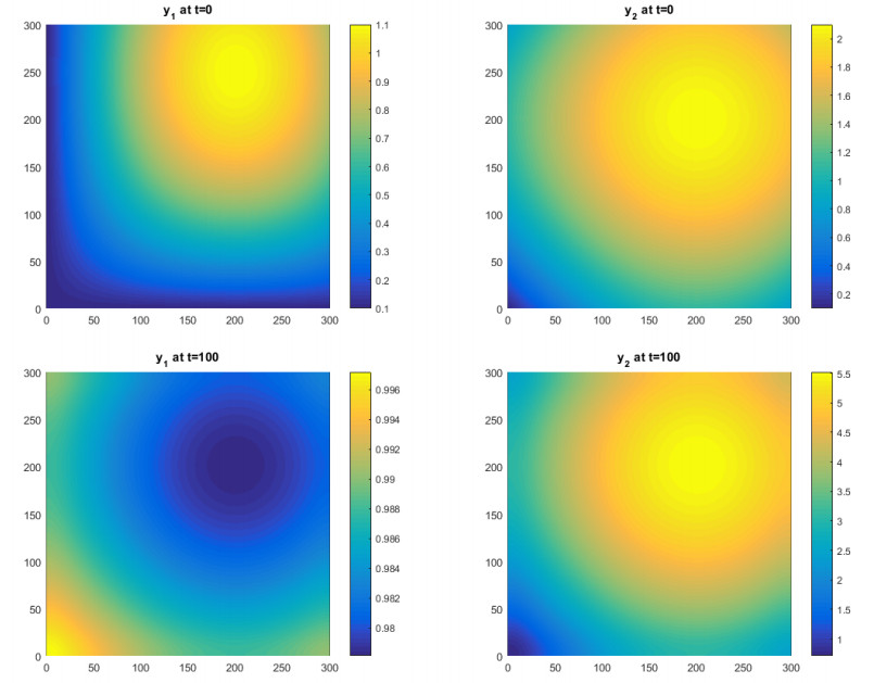
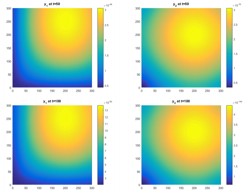
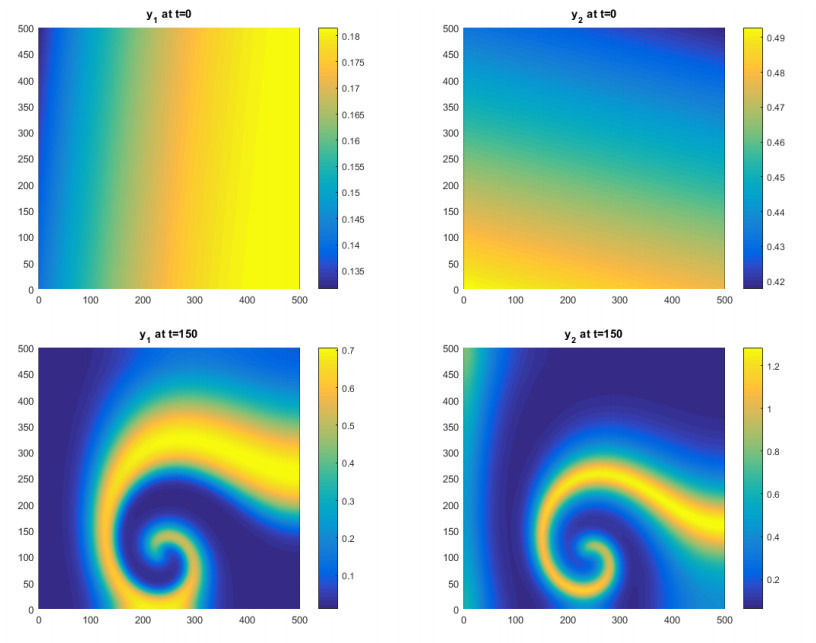
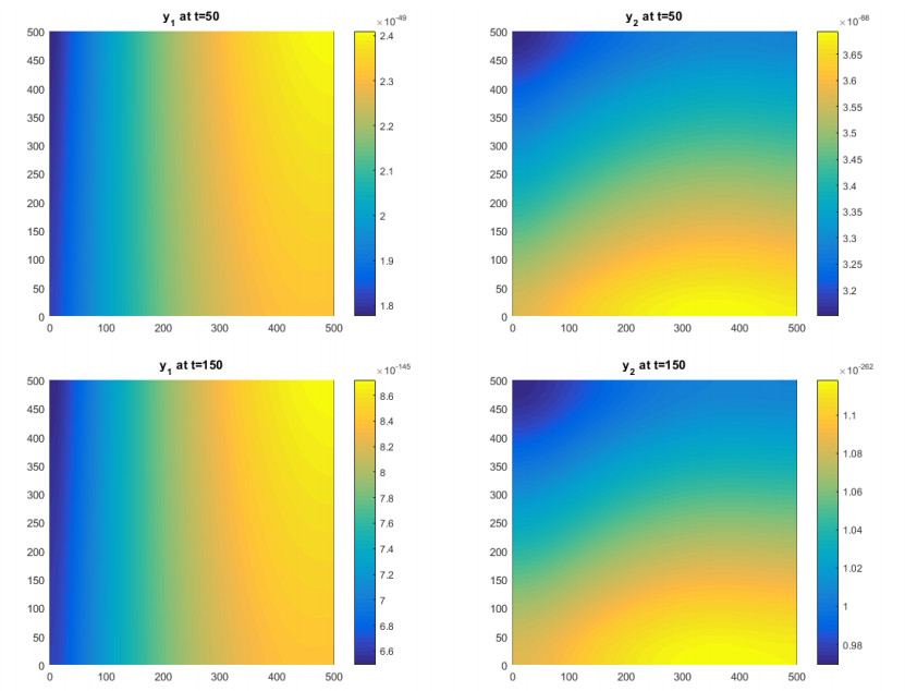
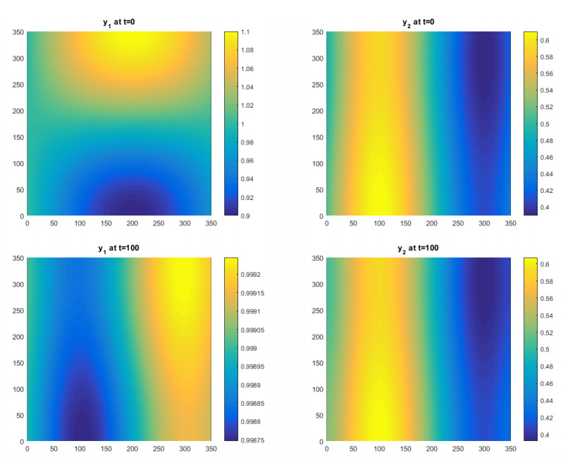
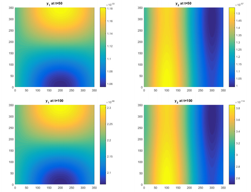
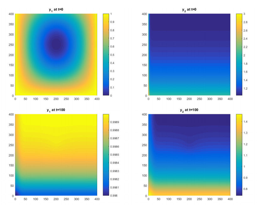
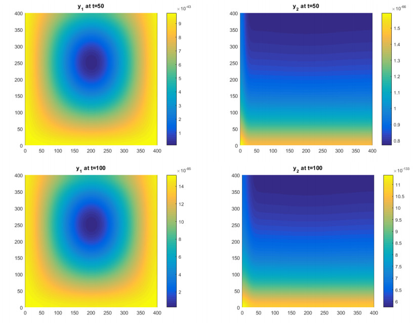
In this paper, we consider a predator–prey model given by a reaction–diffusion system. This model encompasses the classic Holling Ⅰ, Holling Ⅱ, Holling Ⅲ, and Holling Ⅳ functional responses. We investigate the stabilization problem of the considered system using multiplicative controls. By linearizing the system and using the maximum principle, we construct a multiplicative control that exponentially stabilizes the system towards its steady-state solutions. The proposed feedback control allows us to reach a large class of steady-state solutions. The global well-posedness is obtained via Banach fixed point. Applications and numerical simulations to Holling responses Ⅰ, Ⅱ, Ⅲ, and Ⅳ are presented.
Citation: Ilyasse Lamrani, Imad El Harraki, M. A. Aziz-Alaoui, Fatima-Zahrae El Alaoui. Feedback stabilization for prey predator general model with diffusion via multiplicative controls[J]. AIMS Mathematics, 2023, 8(1): 2360-2385. doi: 10.3934/math.2023122
In this paper, we consider a predator–prey model given by a reaction–diffusion system. This model encompasses the classic Holling Ⅰ, Holling Ⅱ, Holling Ⅲ, and Holling Ⅳ functional responses. We investigate the stabilization problem of the considered system using multiplicative controls. By linearizing the system and using the maximum principle, we construct a multiplicative control that exponentially stabilizes the system towards its steady-state solutions. The proposed feedback control allows us to reach a large class of steady-state solutions. The global well-posedness is obtained via Banach fixed point. Applications and numerical simulations to Holling responses Ⅰ, Ⅱ, Ⅲ, and Ⅳ are presented.

| [1] |
N. Apreutesei, G. Dimitriu, On a prey–predator reaction–diffusion system with holling type iii functional response, J. Comput. Appl. Math., 235 (2010), 366–379. https://doi.org/10.1016/j.cam.2010.05.040 doi: 10.1016/j.cam.2010.05.040

|
| [2] |
M. A. Aziz-Alaoui, M. D. Okiye, Boundedness and global stability for a predator-prey model with modified leslie-gower and holling-type ii schemes, Appl. Math. Lett., 16 (2003), 1069–1075. https://doi.org/10.1016/S0893-9659(03)90096-6 doi: 10.1016/S0893-9659(03)90096-6
|
| [3] |
J. M. Ball, J. E. Marsden, M. Slemrod, Controllability for distributed bilinear systems, SIAM J. Control Optim., 20 (1982), 575–597. https://doi.org/10.1137/0320042 doi: 10.1137/0320042
|
| [4] |
L. Berrahmoune, Stabilization and decay estimate for distributed bilinear systems, Syst. Control Lett., 36 (1999), 167–171. https://doi.org/10.1016/S0167-6911(98)00065-6 doi: 10.1016/S0167-6911(98)00065-6
|
| [5] |
R. Bhattacharyya, B. Mukhopadhyay, M. Bandyopadhyay, Diffusion-driven stability analysis of a prey-predator system with holling type-iv functional response, Systems Analysis Modelling Simulation, 43 (2003), 1085–1093. https://doi.org/10.1080/0232929031000150409 doi: 10.1080/0232929031000150409
|
| [6] |
P. N. Brown, Decay to uniform states in ecological interactions, SIAM J. Appl. Math., 38 (1980), 22–37. https://doi.org/10.1137/0138002 doi: 10.1137/0138002
|
| [7] | B. I. Camara, M. A. Aziz-Alaoui, Dynamics of a predator-prey model with diffusion, Dynamics of Continuous, Discrete and Impulsive System, series A, 15 (2008), 897–906. |
| [8] | B. I. Camara, M. A. Aziz-Alaoui, Turing and hopf patterns formation in a predator-prey model with leslie-gowertype functional response, Dynamics of Continuous, Discrete & Impulsive Systems B, 16 (2009), 479–488. |
| [9] |
X. Chen, Y. Qi, M. Wang, A strongly coupled predator–prey system with non-monotonic functional response, Nonlinear Anal.-Theor., 67 (2007), 1966–1979. https://doi.org/10.1016/j.na.2006.08.022 doi: 10.1016/j.na.2006.08.022
|
| [10] |
C. Cosner, A. C. Lazer, Stable coexistence states in the volterra–lotka competition model with diffusion, SIAM J. Appl. Math., 44 (1984), 1112–1132. https://doi.org/10.1137/0144080 doi: 10.1137/0144080
|
| [11] | P. De Mottoni, Qualitative analysis for some quasi-linear parabolic systems, Inst. Math. Pol. Acad. Sci. Zam, 1979. |
| [12] | K.-J. Engel, R. Nagel, S. Brendle, One-parameter semigroups for linear evolution equations, volume 194, Springer, 2000. |
| [13] |
H. I. Freedman, A model of predator-prey dynamics as modified by the action of a parasite, Math. Biosci., 99 (1990), 143–155. https://doi.org/10.1016/0025-5564(90)90001-F doi: 10.1016/0025-5564(90)90001-F
|
| [14] |
M. R. Garvie, Finite-difference schemes for reaction–diffusion equations modeling predator–prey interactions in matlab, B. Math. Biol., 69 (2007), 931–956. https://doi.org/10.1007/s11538-006-9062-3 doi: 10.1007/s11538-006-9062-3
|
| [15] |
M. R. Garvie, C. Trenchea, Spatiotemporal dynamics of two generic predator–prey models, J. Biol. Dynam., 4 (2010), 559–570. https://doi.org/10.1080/17513750903484321 doi: 10.1080/17513750903484321
|
| [16] |
H. P. W. Gottlieb, Eigenvalues of the laplacian with neumann boundary conditions, The ANZIAM Journal, 26 (1985), 293–309. https://doi.org/10.1017/S0334270000004525 doi: 10.1017/S0334270000004525
|
| [17] | A. Y. Khapalov, Controllability of partial differential equations governed by multiplicative controls, Springer, 2010. https://doi.org/10.1007/978-3-642-12413-6 |
| [18] | K. Kishimoto, H. F. Weinberger, The spatial homogeneity of stable equilibria of some reaction-diffusion systems on convex domains, 1988. |
| [19] |
I. Lamrani, I. El Harraki, A. Boutoulout, F.-Z. El Alaoui, Feedback stabilization of bilinear coupled hyperbolic systems, Discrete & Continuous Dynamical Systems-S, 14 (2021), 3641. https://doi.org/10.3934/dcdss.2020434 doi: 10.3934/dcdss.2020434
|
| [20] |
Y. Lou, W.-M. Ni, Diffusion, self-diffusion and cross-diffusion, J. Differ. Equations, 131 (1996), 79–131. https://doi.org/10.1006/jdeq.1996.0157 doi: 10.1006/jdeq.1996.0157
|
| [21] |
T. Ma, X. Meng, T. Hayat, A. Hobiny, Stability analysis and optimal harvesting control of a cross-diffusion prey-predator system, Chaos, Solitons & Fractals, 152 (2021), 111418. https://doi.org/10.1016/j.chaos.2021.111418 doi: 10.1016/j.chaos.2021.111418
|
| [22] |
A. B. Medvinsky, S. V. Petrovskii, I. A. Tikhonova, H. Malchow, B.-L. Li, Spatiotemporal complexity of plankton and fish dynamics, SIAM review, 44 (2002), 311–370. https://doi.org/10.1137/S0036144502404442 doi: 10.1137/S0036144502404442
|
| [23] | S.-Y. Mi, B.-S. Han, Y. Yang, Spatial dynamics of a nonlocal predator–prey model with double mutation, Int. J. Biomath., (2022), 2250035. |
| [24] |
Y. Morita, K. Tachibana, An entire solution to the lotka–volterra competition-diffusion equations, SIAM J. Math. Anal., 40 (2009), 2217–2240. https://doi.org/10.1137/080723715 doi: 10.1137/080723715
|
| [25] | A. Pazy, Semigroups of linear operators and applications to partial differential equations, volume 44, Springer Science & Business Media, 2012. |
| [26] |
J. P. Quinn, Stabilization of bilinear systems by quadratic feedback controls, J. Math. Anal. Appl., 75 (1980), 66–80. https://doi.org/10.1016/0022-247X(80)90306-6 doi: 10.1016/0022-247X(80)90306-6
|
| [27] | J. Smoller, Shock waves and reaction—diffusion equations, volume 258, Springer Science & Business Media, 2012. |
| [28] |
Y. Tian, P. Weng, Stability analysis of diffusive predator–prey model with modified leslie–gower and holling-type iii schemes, Appl. Math. Comput., 218 (2011), 3733–3745. https://doi.org/10.1016/j.amc.2011.09.018 doi: 10.1016/j.amc.2011.09.018
|
| [29] |
W. Walter, Differential inequalities and maximum principles: theory, new methods and applications, Nonlinear Anal.-Theor., 30 (1997), 4695–4711. https://doi.org/10.1016/S0362-546X(96)00259-3 doi: 10.1016/S0362-546X(96)00259-3
|
| [30] |
H. Zhang, Y. Cai, S. Fu, W. Wang, Impact of the fear effect in a prey-predator model incorporating a prey refuge, Appl. Math. Comput., 356 (2019), 328–337. https://doi.org/10.1016/j.amc.2019.03.034 doi: 10.1016/j.amc.2019.03.034
|
| [31] | I. Munteanu, Boundary stabilization of parabolic equations, volume 44, Springer International Publishing, 2019. |
Figures(8)

Ilyasse Lamrani, Imad El Harraki, M. A. Aziz-Alaoui, Fatima-Zahrae El Alaoui. Feedback stabilization for prey predator general model with diffusion via multiplicative controls[J]. AIMS Mathematics, 2023, 8(1): 2360-2385. doi: 10.3934/math.2023122


 DownLoad: