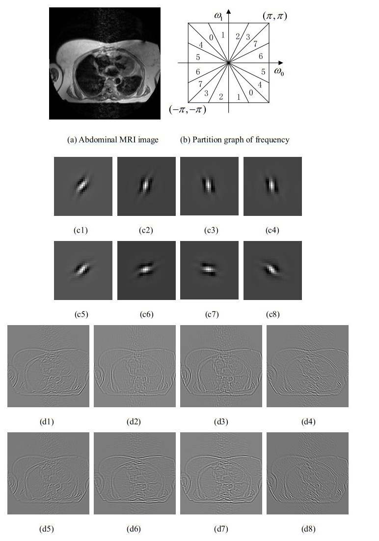
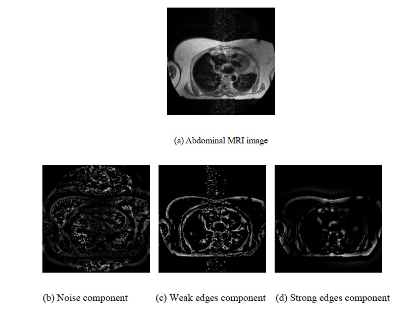
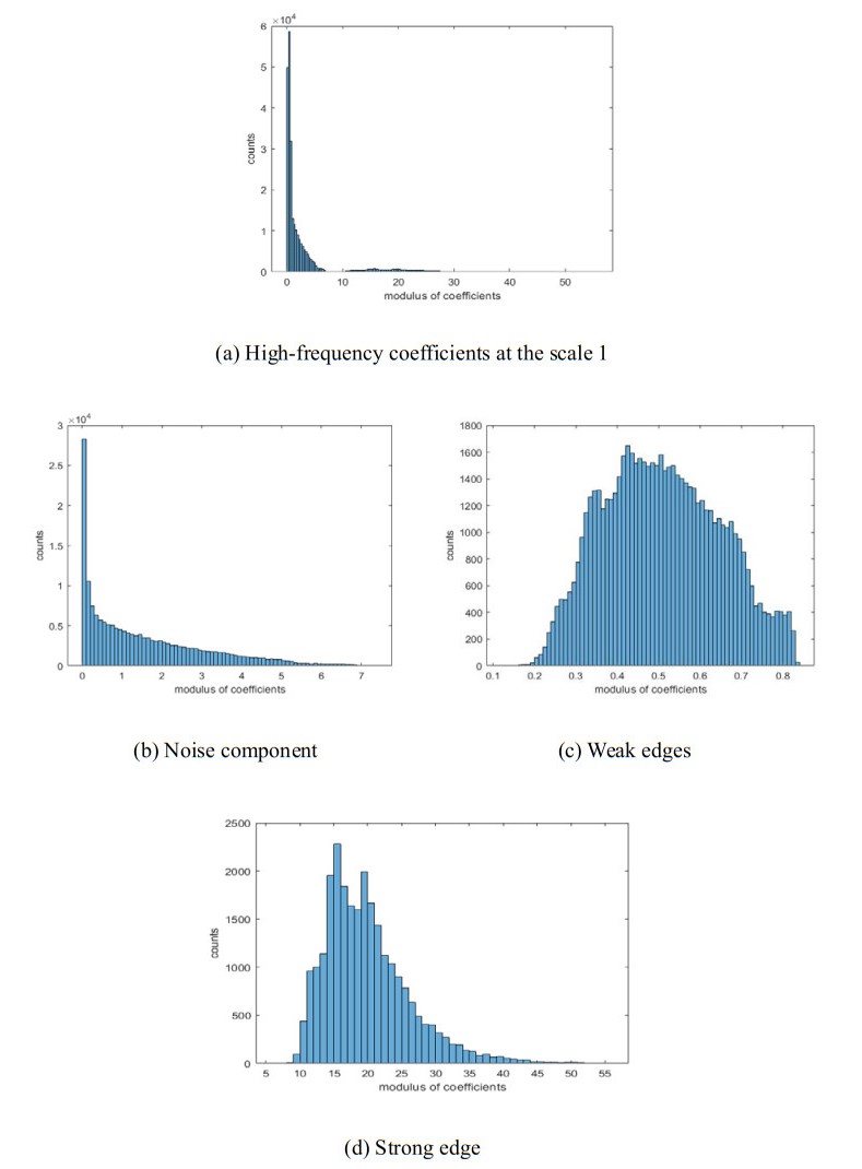
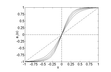
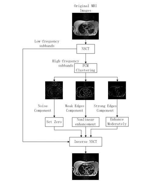
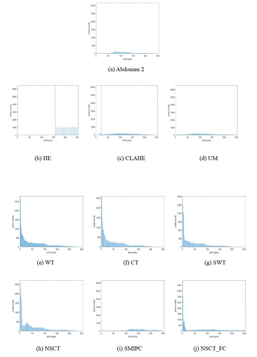
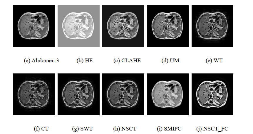
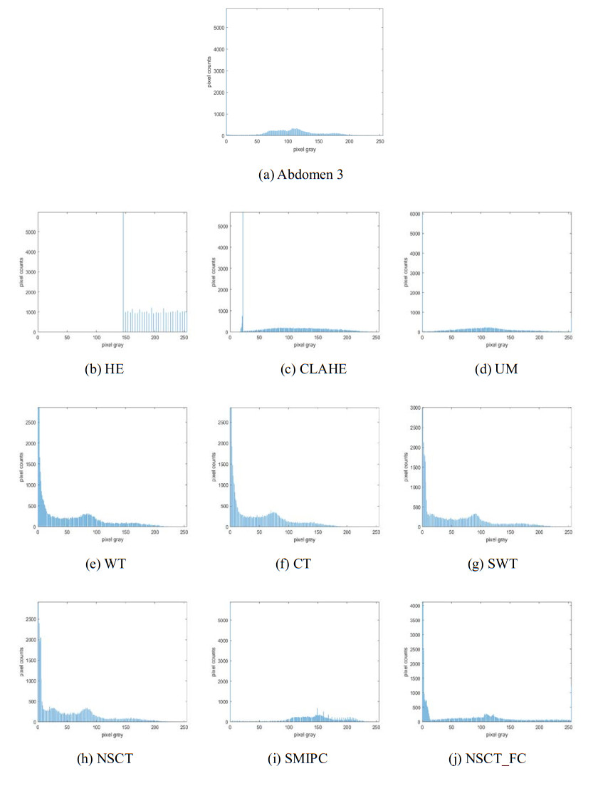
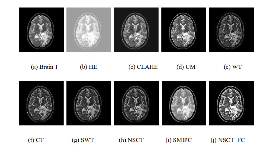
The noise and low clarity in magnetic resonance imaging (MRI) images impede the doctor's diagnosis. An MRI image enhancement method is proposed in the non-subsampled contourlet transform (NSCT) domain. The coefficients of the NSCT are classified as noise component, weak edges component and strong edges component by feature clustering. We modified the transform coefficients to enhance the MRI images. The coefficients corresponding to noise are set to zero, the coefficients corresponding to strong edges are essentially unchanged, and the coefficients corresponding to weak edges are enhanced by a simplified nonlinear gain function. It is shown that the proposed MRI image enhancement method has advantages in visual quality and objective evaluation indexes compared to the state-of-the-art methods.
Citation: Xia Chang, Haixia Zhao, Zhenxia Xue. MRI image enhancement based on feature clustering in the NSCT domain[J]. AIMS Mathematics, 2022, 7(8): 15633-15658. doi: 10.3934/math.2022856
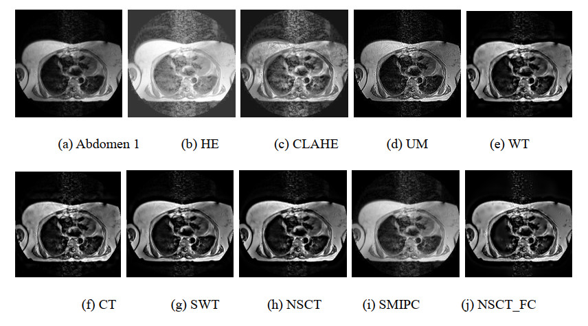
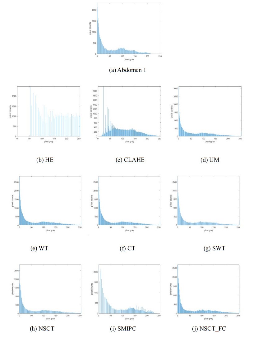
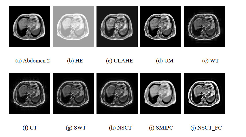
The noise and low clarity in magnetic resonance imaging (MRI) images impede the doctor's diagnosis. An MRI image enhancement method is proposed in the non-subsampled contourlet transform (NSCT) domain. The coefficients of the NSCT are classified as noise component, weak edges component and strong edges component by feature clustering. We modified the transform coefficients to enhance the MRI images. The coefficients corresponding to noise are set to zero, the coefficients corresponding to strong edges are essentially unchanged, and the coefficients corresponding to weak edges are enhanced by a simplified nonlinear gain function. It is shown that the proposed MRI image enhancement method has advantages in visual quality and objective evaluation indexes compared to the state-of-the-art methods.

| [1] |
W. S. Hinshaw, P. A. Bottomley, G. N. Holland, Radiographic thin-section image of the human wrist by nuclear magnetic resonance, Nature, 270 (1977), 722-723. https://doi.org/10.1038/270722a0 doi: 10.1038/270722a0

|
| [2] |
K. H. Wan, S. H. Shi, C. Z. Shao, Y. B. Liu, M. Li, T. S. Hou, et al., An MRI study of psoas major and abdominal large vessels with respect to the X/DLIF approach, Eur. Spine J., 20 (2011), 557-562. https://doi.org/10.7507/1002-1892.20160291 doi: 10.7507/1002-1892.20160291
|
| [3] |
R. H. Wang, J. H. Lv, S. L. Ma, A MRI image segmentation method based on medical semaphore calculating in medical multimedia big data environment, Multimed. Tools Appl., 77 (2018), 9995-10015. https://doi.org/10.1007/s11042-017-4591-3 doi: 10.1007/s11042-017-4591-3
|
| [4] | S. S. Bedi, K. Rati, Various image enhancement techniques-a critical review, Int. J. Adv. Res. Comput. Commun. Eng., 2 (2013), 1605-1609. |
| [5] |
R. Kaur, K. Kaur, Study of Image enhancement techniques in image processing: A review, Int. J. Eng. Manuf., 6 (2016), 38-50. https://doi.org/10.5815/ijem.2016.06.04 doi: 10.5815/ijem.2016.06.04
|
| [6] |
K. Singh, A. Seth, H. S. Sandhu, A comprehensive review of convolutional neural network based image enhancement techniques, IEEE Int. Conf. Syst. Comput. Autom. Netw., 2019, 1-6. https://doi.org/10.1109/ICSCAN.2019.8878706 doi: 10.1109/ICSCAN.2019.8878706
|
| [7] |
R. Hummel, Image enhancement by histogram transformation, Comput. Graphics Image Process., 6 (1997), 184-195. https://doi.org/10.1016/S0146-664X(77)80011-7 doi: 10.1016/S0146-664X(77)80011-7
|
| [8] |
Y. Liu, J. Guo, J. Yu, Contrast enhancement using stratifified parametric-oriented histogram equalization, IEEE T. Circ. Syst. Vid., 27 (2017), 1171-1181. https://doi.org/10.1109/TCSVT.2016.2527338 doi: 10.1109/TCSVT.2016.2527338
|
| [9] | K. Zuiderveld, Contrast limited adaptive histogram equalization, Academic Press Professional, Inc., 1994. https://doi.org/10.1016/B978-0-12-336156-1.50061-6 |
| [10] |
J. Sheeba, S. Parasuraman, K. Amudha, Contrast enhancement and brightness preserving of digital mammograms using fuzzy clipped contrast-limited adaptive histogram equalization algorithm, Appl. Soft Comput., 42 (2016), 167-177. https://doi.org/10.1016/j.asoc.2016.01.039 doi: 10.1016/j.asoc.2016.01.039
|
| [11] |
B. Vikrant, M. Mukul, U. Shabana, Human visual system based unsharp masking for enhancement of mammographic images, J. Comput. Sci., 21 (2017), 387-393. https://doi.org/10.1016/j.jocs.2016.07.015 doi: 10.1016/j.jocs.2016.07.015
|
| [12] |
W. Ye, K. Ma, Blurriness-guided unsharp masking, IEEE T. Image Proces., 27 (2018), 4465-4477. https://doi.org/10.1109/TIP.2018.2838660 doi: 10.1109/TIP.2018.2838660
|
| [13] |
S. K. Chandra, M. K. Bajpai, Fractional mesh-free linear diffusion method for image enhancement and segmentation for automatic tumor classification, Biomed. Signal Proces., 58 (2020), 101841. https://doi.org/10.1016/j.bspc.2019.101841 doi: 10.1016/j.bspc.2019.101841
|
| [14] |
A. R. Al-Shamasneh, H. A. Jalab, S. Palaiahnakote, U. H. Obaidellah, R. W. Ibrahim, M. T. El-Melegy, A new local fractional entropy-based model for kidney MRI image enhancement, Entropy, 20 (2018), 344. https://doi.org/10.3390/e20050344 doi: 10.3390/e20050344
|
| [15] |
Z. Y. Chen, B. R. Abidi, D. L. Page, M. A. Abidi, Gray-level grouping: An automatic method for optimized image contrast enhancement part 1: The basic method, IEEE T. Image Proces., 15 (2006), 2290-2302. https://doi.org/10.1109/TIP.2006.875204 doi: 10.1109/TIP.2006.875204
|
| [16] |
A. Polesel, G. Ramponi, V. J. Mathews, Image enhancement via adaptive unsharp masking, IEEE T. Image Proces., 9 (2000), 505-510. https://doi.org/10.1109/83.826787 doi: 10.1109/83.826787
|
| [17] |
A. M. Chikhalikar, N. V. Dharwadkar, Model for enhancement and segmentation of magnetic resonance images for brain tumor classification, Pattern Recog. Image, 31 (2021), 49-59. https://doi.org/10.1134/S1054661821010065 doi: 10.1134/S1054661821010065
|
| [18] |
L. Cao, H. Q Li, Y. J. Zhang, Retinal image enhancement using low-pass filtering and α-rooting, Signal Proces., 170 (2020), 107445. https://doi.org/10.1016/j.sigpro.2019.107445 doi: 10.1016/j.sigpro.2019.107445
|
| [19] |
D. Wei, Z. Wang. Channel rearrangement multi-branch network for image super-resolution, Digit. Signal Proces., 120 (2022), 103254. https://doi.org/10.1016/j.dsp.2021.103254 doi: 10.1016/j.dsp.2021.103254
|
| [20] |
D. Wei, Y. M. Li, Convolution and multichannel sampling for the offset linear canonical transform and their applications, IEEE T. Signal Proces., 67 (2019), 6009-6024. https://doi.org/10.1109/TSP.2019.2951191 doi: 10.1109/TSP.2019.2951191
|
| [21] |
D. Wei, Linear canonical stockwell transform: Theory and applications, IEEE T. Signal Proces., 70 (2022), 1333-1347. https://doi.org/10.1109/TSP.2022.3152402 doi: 10.1109/TSP.2022.3152402
|
| [22] |
D. L. Donoho, A. G. Flesia, Can recent innovations in harmonic analysis 'explain' key findings in natural image statistics? Network-Comp. Neural, 12 (2001), 371-393. https://doi.org/10.1080/net.12.3.371.393 doi: 10.1080/net.12.3.371.393
|
| [23] |
A. L. Cunha, J. Zhou, M. N. Do, The nonsubsampled contourlet transform: Theory, design, and applications, IEEE T. Image Proces., 15 (2006), 3089-3101. https://doi.org/10.1109/TIP.2006.877507 doi: 10.1109/TIP.2006.877507
|
| [24] |
X. Chang, L. C. Jiao, F. Liu, Y. H Sha, SAR Image despeckling using scale mixtures of gaussians in the nonsubsampled contourlet domain, Chinese J. Electron., 24 (2015), 205-211. https://doi.org/10.1049/cje.2015.01.034 doi: 10.1049/cje.2015.01.034
|
| [25] |
M. M. Hasan, M. M. Hossain, S. Mia, A. M. Shmed, R. M. Mahman, A combined approach of non-subsampled contourlet transform and convolutional neural network to detect gastrointestinal polyp, Multimed. Tools Appl., 2022, 9949-9968 https://doi.org/10.1007/s11042-022-12250-2 doi: 10.1007/s11042-022-12250-2
|
| [26] |
I. Gath, A. B. Geva, Unsupervised optimal fuzzy clustering, IEEE T. Pattern Anal., 11 (1989), 773-780. https://doi.org/10.1109/34.192473 doi: 10.1109/34.192473
|
| [27] |
T. B. Ren, H. H. Wang, H. L. Feng, C. S. Xu, G. S. Liu, P. Ding, Study on the improved fuzzy clustering algorithm and its application in brain image segmentation, Appl. Soft Comput., 81 (2019), 105503. https://doi.org/10.1016/j.asoc.2019.105503 doi: 10.1016/j.asoc.2019.105503
|
| [28] |
A. F. Laine, X. Zong, A multiscale sub-octave wavelet transform for de-noising and enhancement, Wavelet Appl. Signal Image Proces. IV, 2825 (1996), 238-249. https://doi.org/10.1117/12.255235 doi: 10.1117/12.255235
|
| [29] |
R. E. Glenn, L. Demetrio, M. P. Vishal, Directional multiscale processing of images using wavelets with composite dilations, J. Math. Imaging Vis., 48 (2014), 13-34. https://doi.org/10.1007/s10851-012-0385-4 doi: 10.1007/s10851-012-0385-4
|
| [30] | Z. Al-Ameen, Contrast enhancement of medical images using statistical methods with image processing concepts, IEEE Publisher, Erbil, Iraq, 2020,169-173. https://doi.org/10.1109/IEC49899.2020.9122925 |
| [31] |
A. Cohen, I. Daubechies, Non-separable bidimensional wavelet bases, Rev. Mat. Iberoam., 9 (1993), 51-137. https://doi.org/10.4171/RMI/133 doi: 10.4171/RMI/133
|
Figures(15) / Tables(7)

Xia Chang, Haixia Zhao, Zhenxia Xue. MRI image enhancement based on feature clustering in the NSCT domain[J]. AIMS Mathematics, 2022, 7(8): 15633-15658. doi: 10.3934/math.2022856


 DownLoad: